Machine Learning Generative verses discriminative classifier Eric Xing

Machine Learning Generative verses discriminative classifier Eric Xing Lecture 2, August 12, 2010 Reading: © Eric Xing @ CMU, 2006 -2010

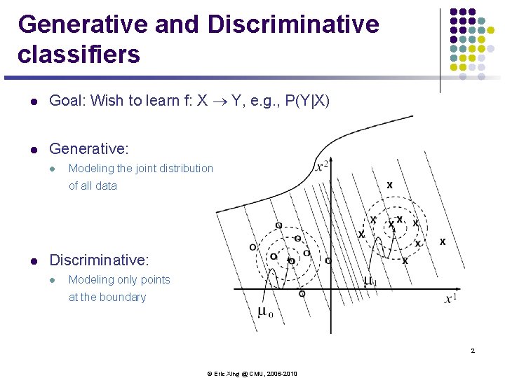
Generative and Discriminative classifiers l Goal: Wish to learn f: X ® Y, e. g. , P(Y|X) l Generative: l Modeling the joint distribution of all data l Discriminative: l Modeling only points at the boundary 2 © Eric Xing @ CMU, 2006 -2010

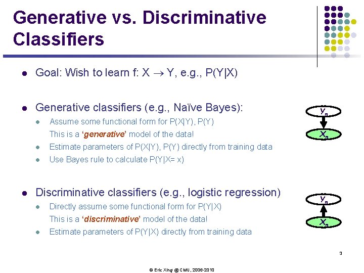
Generative vs. Discriminative Classifiers l Goal: Wish to learn f: X ® Y, e. g. , P(Y|X) l Generative classifiers (e. g. , Naïve Bayes): l Assume some functional form for P(X|Y), P(Y) This is a ‘generative’ model of the data! l l Estimate parameters of P(X|Y), P(Y) directly from training data l Use Bayes rule to calculate P(Y|X= x) Discriminative classifiers (e. g. , logistic regression) l Directly assume some functional form for P(Y|X) This is a ‘discriminative’ model of the data! l Estimate parameters of P(Y|X) directly from training data Yn Xn 3 © Eric Xing @ CMU, 2006 -2010

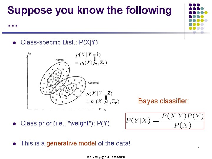
Suppose you know the following … l Class-specific Dist. : P(X|Y) Bayes classifier: l Class prior (i. e. , "weight"): P(Y) l This is a generative model of the data! © Eric Xing @ CMU, 2006 -2010 4

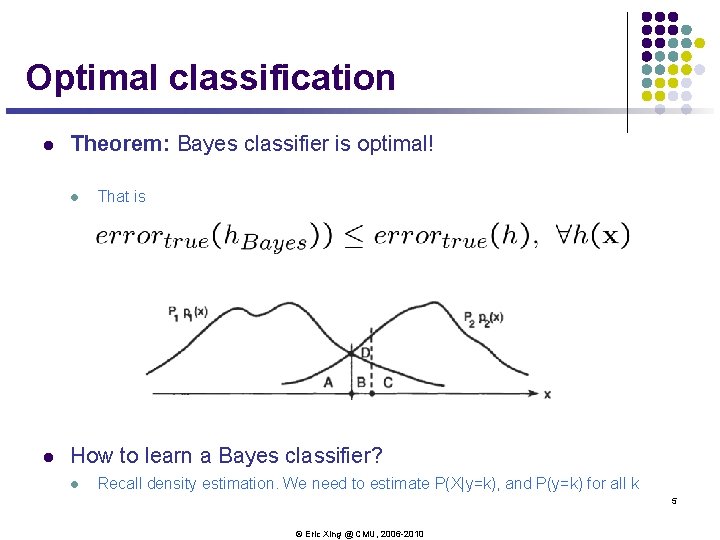
Optimal classification l Theorem: Bayes classifier is optimal! l l That is How to learn a Bayes classifier? l Recall density estimation. We need to estimate P(X|y=k), and P(y=k) for all k 5 © Eric Xing @ CMU, 2006 -2010

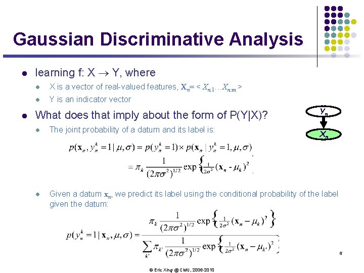
Gaussian Discriminative Analysis l l learning f: X ® Y, where l X is a vector of real-valued features, Xn= < Xn, 1…Xn, m > l Y is an indicator vector What does that imply about the form of P(Y|X)? Yn l The joint probability of a datum and its label is: l Given a datum xn, we predict its label using the conditional probability of the label given the datum: Xn 6 © Eric Xing @ CMU, 2006 -2010

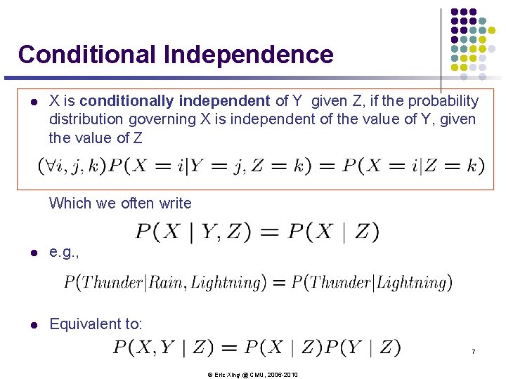
Conditional Independence l X is conditionally independent of Y given Z, if the probability distribution governing X is independent of the value of Y, given the value of Z Which we often write l e. g. , l Equivalent to: 7 © Eric Xing @ CMU, 2006 -2010

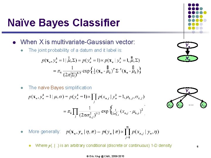
Naïve Bayes Classifier l When X is multivariate-Gaussian vector: l Yn The joint probability of a datum and it label is: Xn l The naïve Bayes simplification Yn Xn, 1 l Xn, 2 … Xn, m More generally: l Where p(. |. ) is an arbitrary conditional (discrete or continuous) 1 -D density © Eric Xing @ CMU, 2006 -2010 8

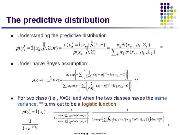
The predictive distribution l Understanding the predictive distribution l Under naïve Bayes assumption: l For two class (i. e. , K=2), and when the two classes haves the same variance, ** turns out to be a logistic function 9 © Eric Xing @ CMU, 2006 -2010

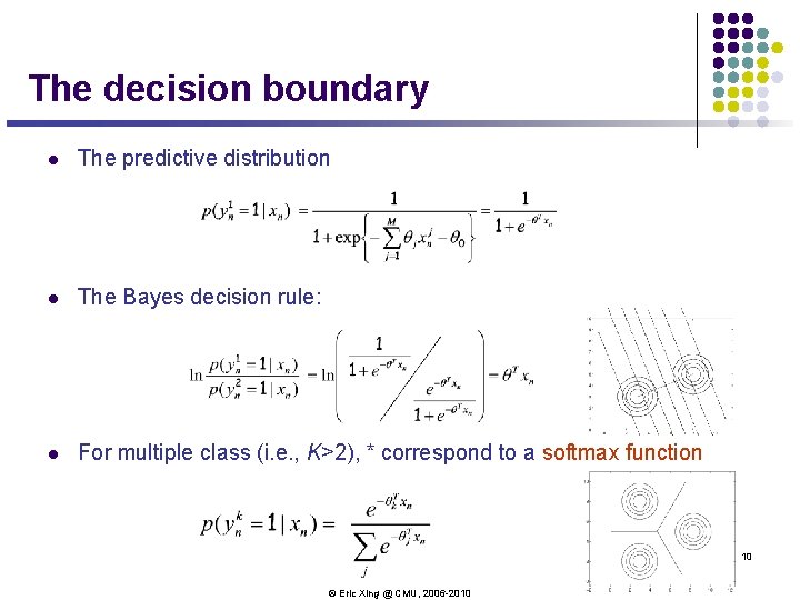
The decision boundary l The predictive distribution l The Bayes decision rule: l For multiple class (i. e. , K>2), * correspond to a softmax function 10 © Eric Xing @ CMU, 2006 -2010

Generative vs. Discriminative Classifiers l Goal: Wish to learn f: X ® Y, e. g. , P(Y|X) l Generative classifiers (e. g. , Naïve Bayes): l Assume some functional form for P(X|Y), P(Y) This is a ‘generative’ model of the data! l l Estimate parameters of P(X|Y), P(Y) directly from training data l Use Bayes rule to calculate P(Y|X= x) Discriminative classifiers: l Directly assume some functional form for P(Y|X) This is a ‘discriminative’ model of the data! l Estimate parameters of P(Y|X) directly from training data Yi Xi 11 © Eric Xing @ CMU, 2006 -2010

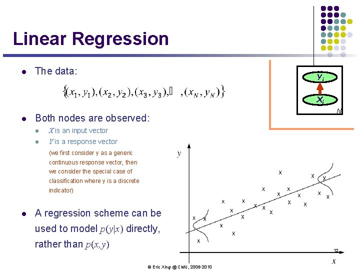
Linear Regression l The data: Yi Xi l Both nodes are observed: l X is an input vector l Y is a response vector N (we first consider y as a generic continuous response vector, then we consider the special case of classification where y is a discrete indicator) l A regression scheme can be used to model p(y|x) directly, rather than p(x, y) 12 © Eric Xing @ CMU, 2006 -2010

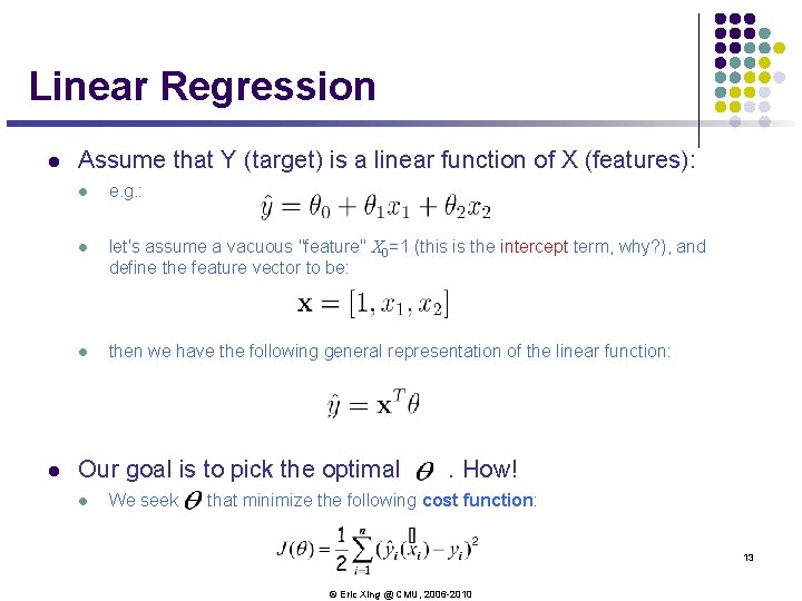
Linear Regression l l Assume that Y (target) is a linear function of X (features): l e. g. : l let's assume a vacuous "feature" X 0=1 (this is the intercept term, why? ), and define the feature vector to be: l then we have the following general representation of the linear function: Our goal is to pick the optimal l We seek . How! that minimize the following cost function: 13 © Eric Xing @ CMU, 2006 -2010

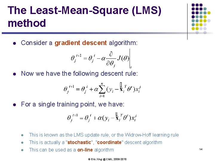
The Least-Mean-Square (LMS) method l Consider a gradient descent algorithm: l Now we have the following descent rule: l For a single training point, we have: l This is known as the LMS update rule, or the Widrow-Hoff learning rule l This is actually a "stochastic", "coordinate" descent algorithm l This can be used as a on-line algorithm © Eric Xing @ CMU, 2006 -2010 14

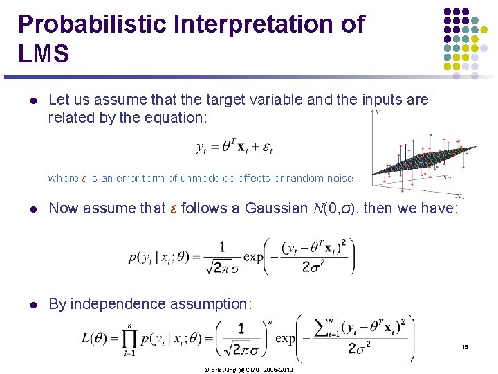
Probabilistic Interpretation of LMS l Let us assume that the target variable and the inputs are related by the equation: where ε is an error term of unmodeled effects or random noise l Now assume that ε follows a Gaussian N(0, σ), then we have: l By independence assumption: 15 © Eric Xing @ CMU, 2006 -2010

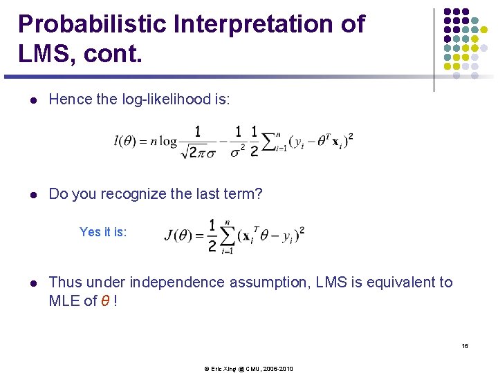
Probabilistic Interpretation of LMS, cont. l Hence the log-likelihood is: l Do you recognize the last term? Yes it is: l Thus under independence assumption, LMS is equivalent to MLE of θ ! 16 © Eric Xing @ CMU, 2006 -2010

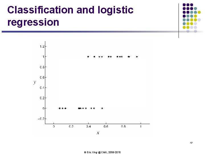
Classification and logistic regression 17 © Eric Xing @ CMU, 2006 -2010

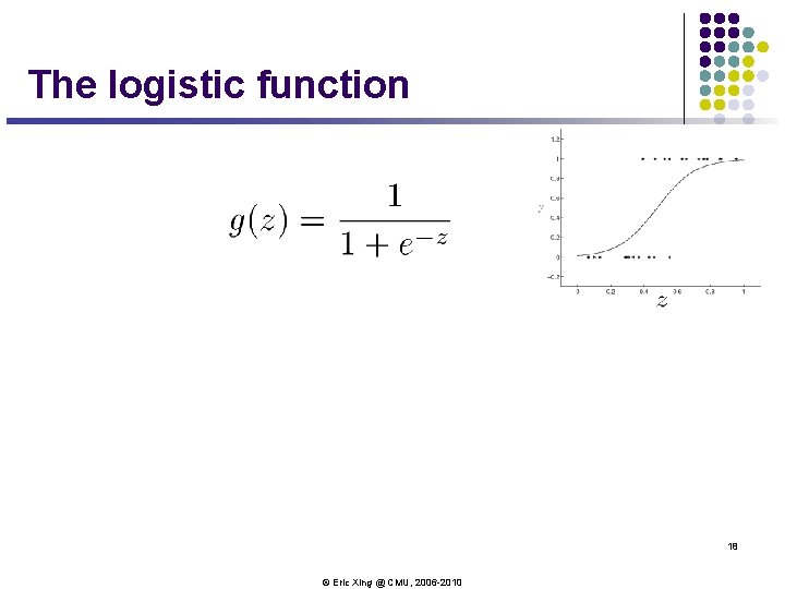
The logistic function 18 © Eric Xing @ CMU, 2006 -2010

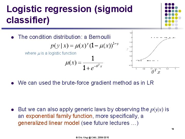
Logistic regression (sigmoid classifier) l The condition distribution: a Bernoulli where m is a logistic function l We can used the brute-force gradient method as in LR l But we can also apply generic laws by observing the p(y|x) is an exponential family function, more specifically, a generalized linear model (see future lectures …) 19 © Eric Xing @ CMU, 2006 -2010

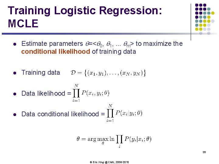
Training Logistic Regression: MCLE l Estimate parameters q=<q 0, q 1, . . . qm> to maximize the conditional likelihood of training data l Training data l Data likelihood = l Data conditional likelihood = 20 © Eric Xing @ CMU, 2006 -2010

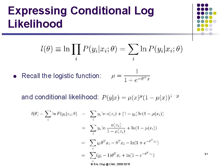
Expressing Conditional Log Likelihood l Recall the logistic function: and conditional likelihood: 21 © Eric Xing @ CMU, 2006 -2010

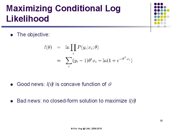
Maximizing Conditional Log Likelihood l The objective: l Good news: l(q) is concave function of q l Bad news: no closed-form solution to maximize l(q) 22 © Eric Xing @ CMU, 2006 -2010

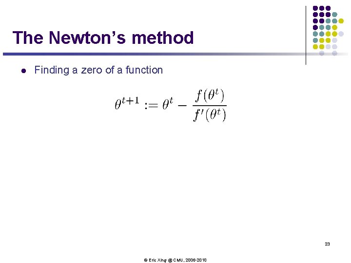
The Newton’s method l Finding a zero of a function 23 © Eric Xing @ CMU, 2006 -2010

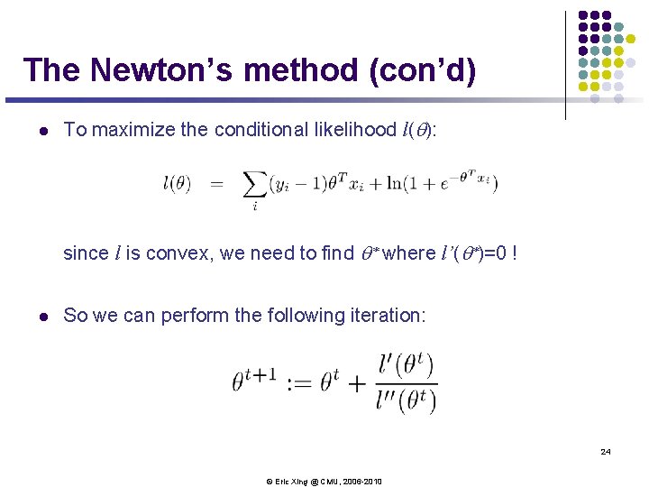
The Newton’s method (con’d) l To maximize the conditional likelihood l(q): since l is convex, we need to find q* where l’(q*)=0 ! l So we can perform the following iteration: 24 © Eric Xing @ CMU, 2006 -2010

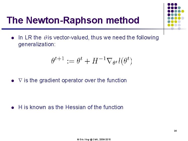
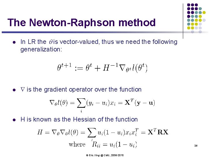
The Newton-Raphson method l In LR the q is vector-valued, thus we need the following generalization: l Ñ is the gradient operator over the function l H is known as the Hessian of the function 25 © Eric Xing @ CMU, 2006 -2010

The Newton-Raphson method l In LR the q is vector-valued, thus we need the following generalization: l Ñ is the gradient operator over the function l H is known as the Hessian of the function 26 © Eric Xing @ CMU, 2006 -2010

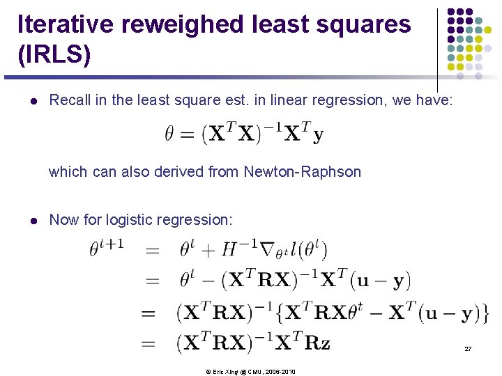
Iterative reweighed least squares (IRLS) l Recall in the least square est. in linear regression, we have: which can also derived from Newton-Raphson l Now for logistic regression: 27 © Eric Xing @ CMU, 2006 -2010

Generative vs. Discriminative Classifiers l Goal: Wish to learn f: X ® Y, e. g. , P(Y|X) l Generative classifiers (e. g. , Naïve Bayes): l Assume some functional form for P(X|Y), P(Y) This is a ‘generative’ model of the data! l l Estimate parameters of P(X|Y), P(Y) directly from training data l Use Bayes rule to calculate P(Y|X= x) Discriminative classifiers: l Directly assume some functional form for P(Y|X) This is a ‘discriminative’ model of the data! l Estimate parameters of P(Y|X) directly from training data Yi Xi 28 © Eric Xing @ CMU, 2006 -2010

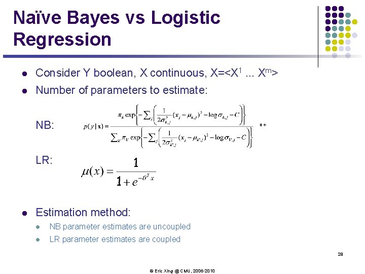
Naïve Bayes vs Logistic Regression l Consider Y boolean, X continuous, X=<X 1. . . Xm> l Number of parameters to estimate: NB: LR: l Estimation method: l NB parameter estimates are uncoupled l LR parameter estimates are coupled 29 © Eric Xing @ CMU, 2006 -2010

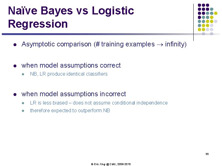
Naïve Bayes vs Logistic Regression l Asymptotic comparison (# training examples ® infinity) l when model assumptions correct l l NB, LR produce identical classifiers when model assumptions incorrect l LR is less biased – does not assume conditional independence l therefore expected to outperform NB 30 © Eric Xing @ CMU, 2006 -2010

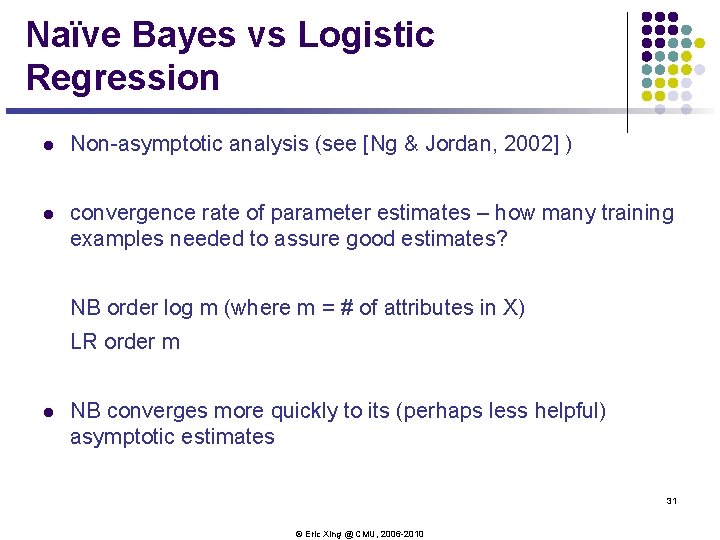
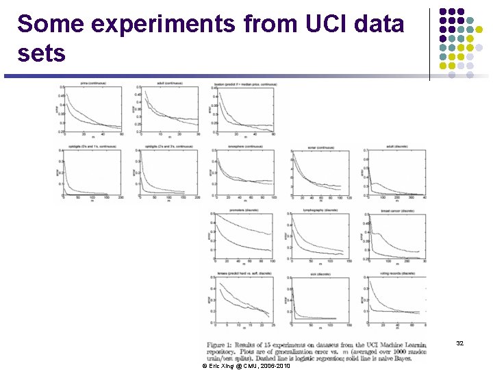
Naïve Bayes vs Logistic Regression l Non-asymptotic analysis (see [Ng & Jordan, 2002] ) l convergence rate of parameter estimates – how many training examples needed to assure good estimates? NB order log m (where m = # of attributes in X) LR order m l NB converges more quickly to its (perhaps less helpful) asymptotic estimates 31 © Eric Xing @ CMU, 2006 -2010

Some experiments from UCI data sets 32 © Eric Xing @ CMU, 2006 -2010

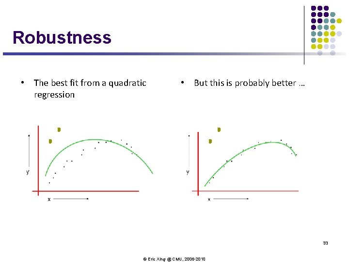
Robustness • The best fit from a quadratic regression • But this is probably better … 33 © Eric Xing @ CMU, 2006 -2010

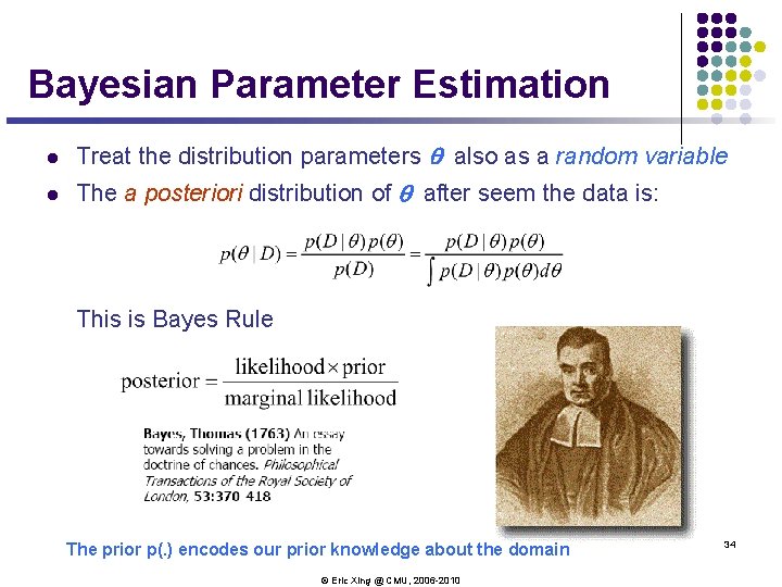
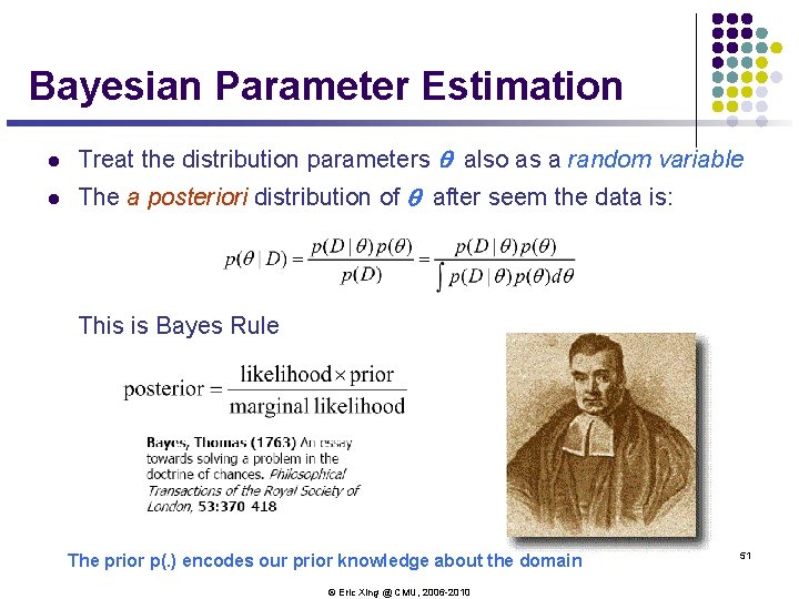
Bayesian Parameter Estimation l Treat the distribution parameters q also as a random variable l The a posteriori distribution of q after seem the data is: This is Bayes Rule The prior p(. ) encodes our prior knowledge about the domain © Eric Xing @ CMU, 2006 -2010 34

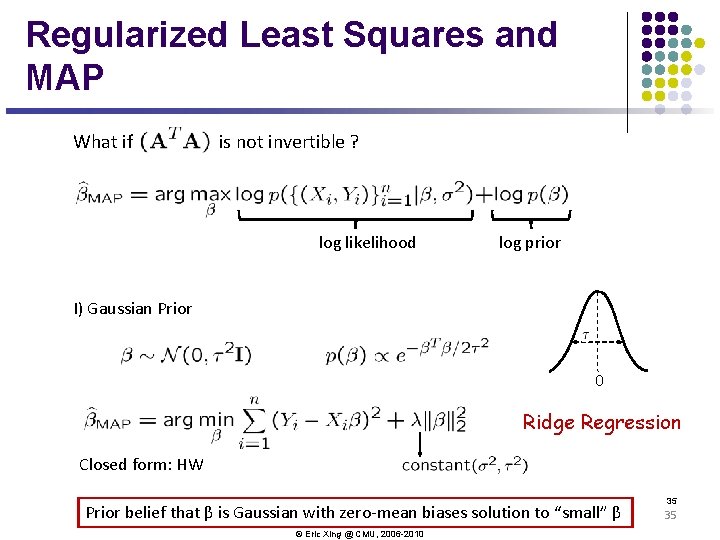
Regularized Least Squares and MAP What if is not invertible ? log likelihood log prior I) Gaussian Prior 0 Ridge Regression Closed form: HW Prior belief that β is Gaussian with zero-mean biases solution to “small” β © Eric Xing @ CMU, 2006 -2010 35 35

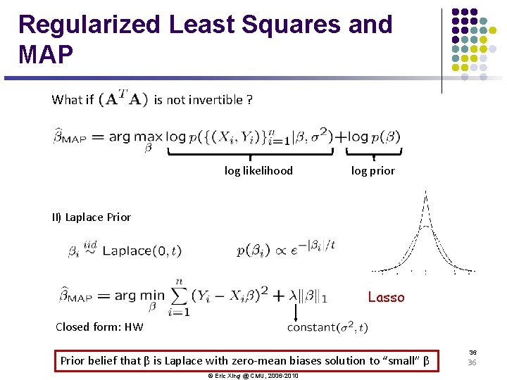
Regularized Least Squares and MAP What if is not invertible ? log likelihood log prior II) Laplace Prior Lasso Closed form: HW Prior belief that β is Laplace with zero-mean biases solution to “small” β © Eric Xing @ CMU, 2006 -2010 36 36

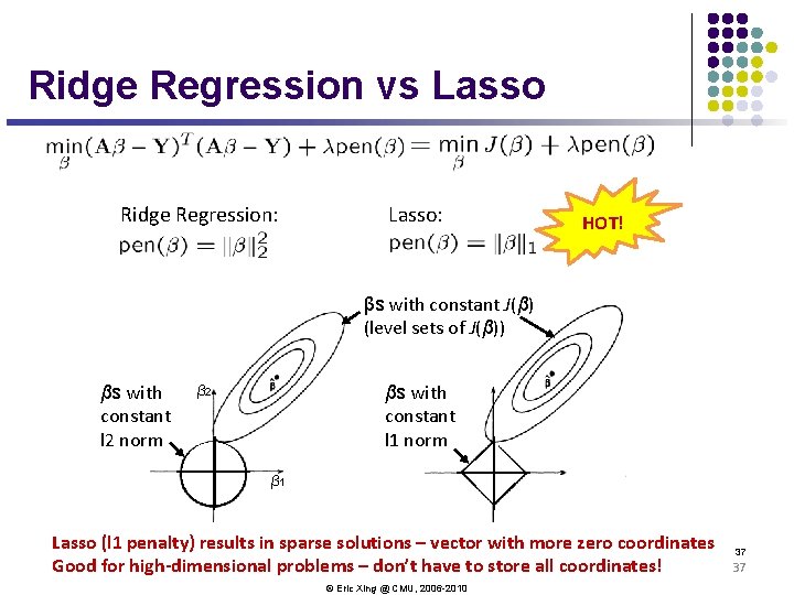
Ridge Regression vs Lasso Ridge Regression: Lasso: HOT! βs with constant J(β) (level sets of J(β)) βs with constant l 2 norm βs with constant l 1 norm β 2 β 1 Lasso (l 1 penalty) results in sparse solutions – vector with more zero coordinates Good for high-dimensional problems – don’t have to store all coordinates! © Eric Xing @ CMU, 2006 -2010 37 37

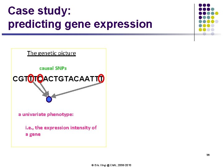
Case study: predicting gene expression The genetic picture causal SNPs CGTTTCACTGTACAATTT a univariate phenotype: i. e. , the expression intensity of a gene 38 © Eric Xing @ CMU, 2006 -2010

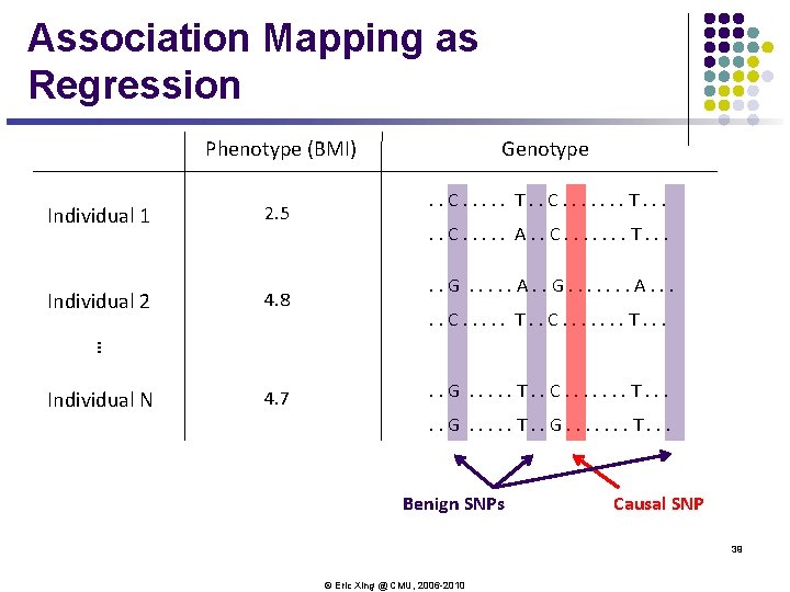
Association Mapping as Regression Phenotype (BMI) 2. 5 Individual 2 4. 8 . . C. . . T. . C. . . . T. . . C. . . A. . C. . . . T. . . G. . . A. . G. . . . A. . . C. . . T. . C. . . . T. . . … Individual 1 Genotype Individual N 4. 7 . . G. . . T. . C. . . . T. . . G. . . T. . G. . . . T. . . Benign SNPs Causal SNP 39 © Eric Xing @ CMU, 2006 -2010

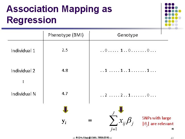
Association Mapping as Regression Genotype Individual 1 2. 5 . . 0. . . 1. . 0. . . Individual 2 4. 8 . . 1. . . 4. 7 . . 2. . 1. . . . 0. . . … Phenotype (BMI) Individual N yi = SNPs with large |βj| are relevant 40 © Eric Xing @ CMU, 2006 -2010

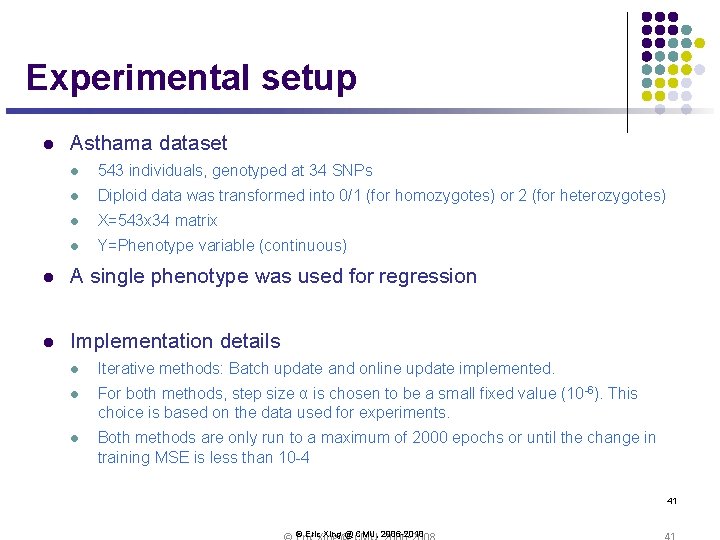
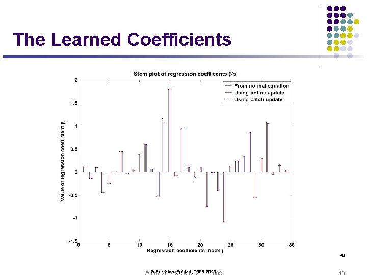
Experimental setup l Asthama dataset l 543 individuals, genotyped at 34 SNPs l Diploid data was transformed into 0/1 (for homozygotes) or 2 (for heterozygotes) l X=543 x 34 matrix l Y=Phenotype variable (continuous) l A single phenotype was used for regression l Implementation details l Iterative methods: Batch update and online update implemented. l For both methods, step size α is chosen to be a small fixed value (10 -6). This choice is based on the data used for experiments. l Both methods are only run to a maximum of 2000 epochs or until the change in training MSE is less than 10 -4 41 © Eric Xing @ CMU, 2006 -2010

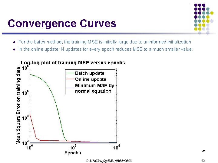
Convergence Curves l For the batch method, the training MSE is initially large due to uninformed initialization l In the online update, N updates for every epoch reduces MSE to a much smaller value. 42 © Eric 2006 -2008 © Eric. Xing@ @ CMU, 2006 -2010 42

The Learned Coefficients 43 © Eric Xing @ CMU, 2006 -2010

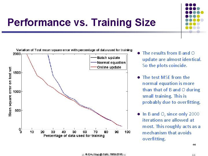
Performance vs. Training Size l The results from B and O update are almost identical. So the plots coincide. l The test MSE from the normal equation is more than that of B and O during small training. This is probably due to overfitting. l In B and O, since only 2000 iterations are allowed at most. This roughly acts as a mechanism that avoids overfitting. 44 © Eric Xing @ CMU, 2006 -2010

Summary l l l Naïve Bayes classifier l What’s the assumption l Why we use it l How do we learn it Logistic regression l Functional form follows from Naïve Bayes assumptions l For Gaussian Naïve Bayes assuming variance l For discrete-valued Naïve Bayes too l But training procedure picks parameters without the conditional independence assumption Gradient ascent/descent l l – General approach when closed-form solutions unavailable Generative vs. Discriminative classifiers l – Bias vs. variance tradeoff 45 © Eric Xing @ CMU, 2006 -2010

Appendix 46 © Eric Xing @ CMU, 2006 -2010

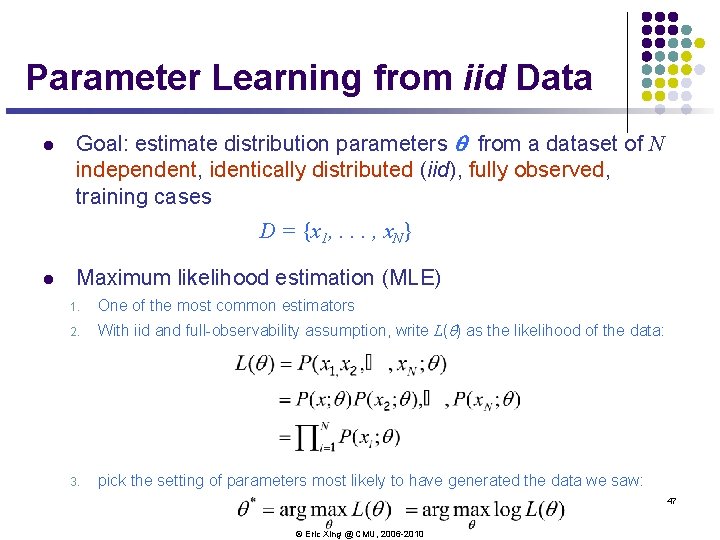
Parameter Learning from iid Data l Goal: estimate distribution parameters q from a dataset of N independent, identically distributed (iid), fully observed, training cases D = {x 1, . . . , x. N} l Maximum likelihood estimation (MLE) 1. One of the most common estimators 2. With iid and full-observability assumption, write L(q) as the likelihood of the data: 3. pick the setting of parameters most likely to have generated the data we saw: 47 © Eric Xing @ CMU, 2006 -2010

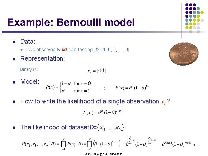
Example: Bernoulli model l Data: l l We observed N iid coin tossing: D={1, 0, 1, …, 0} Representation: Binary r. v: l Model: l How to write the likelihood of a single observation xi ? l The likelihood of dataset. D={x 1, …, x. N}: 48 © Eric Xing @ CMU, 2006 -2010

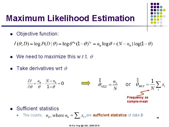
Maximum Likelihood Estimation l Objective function: l We need to maximize this w. r. t. q l Take derivatives wrt q or Frequency as sample mean l Sufficient statistics l The counts, are sufficient statistics of data D © Eric Xing @ CMU, 2006 -2010 49

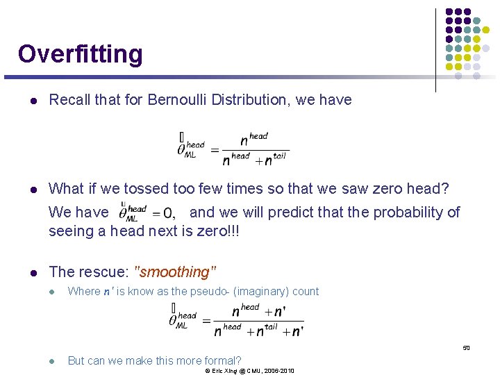
Overfitting l Recall that for Bernoulli Distribution, we have l What if we tossed too few times so that we saw zero head? We have and we will predict that the probability of seeing a head next is zero!!! l The rescue: "smoothing" l Where n' is know as the pseudo- (imaginary) count 50 l But can we make this more formal? © Eric Xing @ CMU, 2006 -2010

Bayesian Parameter Estimation l Treat the distribution parameters q also as a random variable l The a posteriori distribution of q after seem the data is: This is Bayes Rule The prior p(. ) encodes our prior knowledge about the domain © Eric Xing @ CMU, 2006 -2010 51

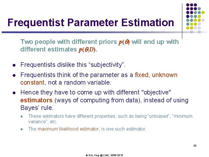
Frequentist Parameter Estimation Two people with different priors p(q) will end up with different estimates p(q|D). l Frequentists dislike this “subjectivity”. l Frequentists think of the parameter as a fixed, unknown constant, not a random variable. l Hence they have to come up with different "objective" estimators (ways of computing from data), instead of using Bayes’ rule. l These estimators have different properties, such as being “unbiased”, “minimum variance”, etc. l The maximum likelihood estimator, is one such estimator. 52 © Eric Xing @ CMU, 2006 -2010

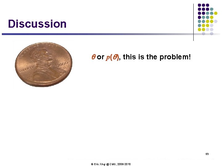
Discussion q or p(q), this is the problem! Bayesians know it 53 © Eric Xing @ CMU, 2006 -2010

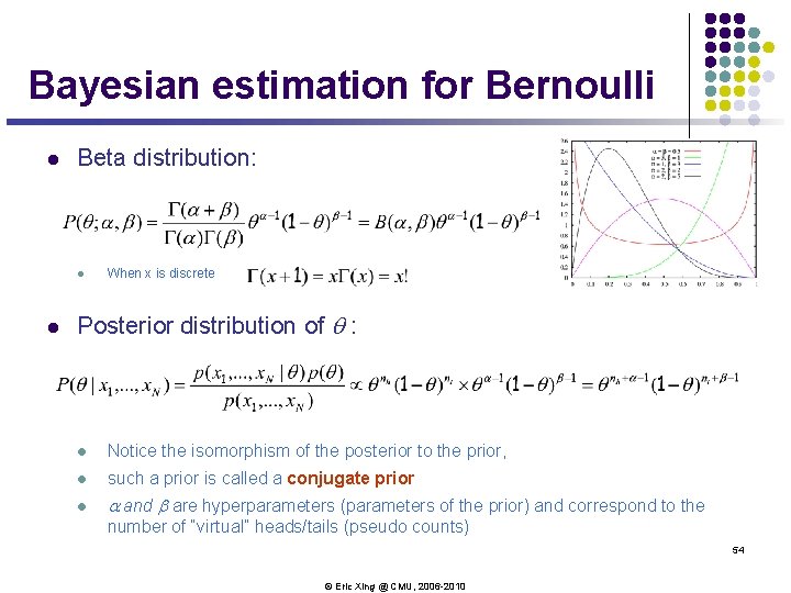
Bayesian estimation for Bernoulli l Beta distribution: l l When x is discrete Posterior distribution of q : l Notice the isomorphism of the posterior to the prior, l such a prior is called a conjugate prior l a and b are hyperparameters (parameters of the prior) and correspond to the number of “virtual” heads/tails (pseudo counts) 54 © Eric Xing @ CMU, 2006 -2010

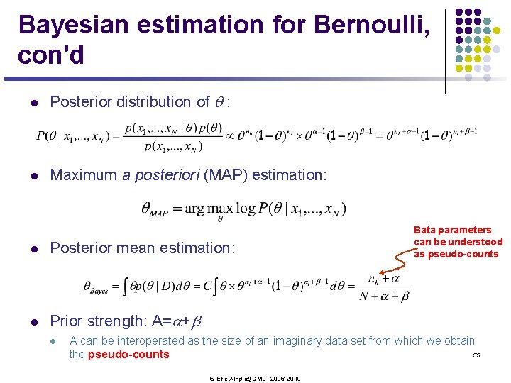
Bayesian estimation for Bernoulli, con'd l Posterior distribution of q : l Maximum a posteriori (MAP) estimation: l Posterior mean estimation: l Prior strength: A=a+b l Bata parameters can be understood as pseudo-counts A can be interoperated as the size of an imaginary data set from which we obtain 55 the pseudo-counts © Eric Xing @ CMU, 2006 -2010

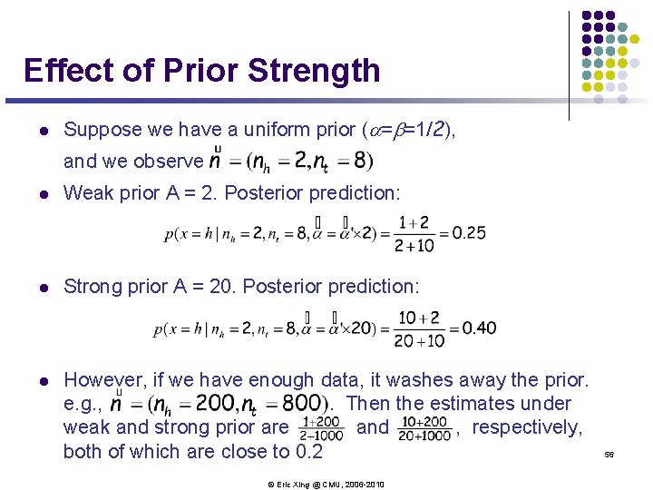
Effect of Prior Strength l Suppose we have a uniform prior (a=b=1/2), and we observe l Weak prior A = 2. Posterior prediction: l Strong prior A = 20. Posterior prediction: l However, if we have enough data, it washes away the prior. e. g. , . Then the estimates under weak and strong prior are and , respectively, both of which are close to 0. 2 © Eric Xing @ CMU, 2006 -2010 56

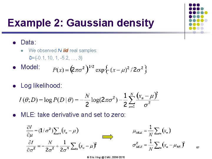
Example 2: Gaussian density l Data: l We observed N iid real samples: D={-0. 1, 10, 1, -5. 2, …, 3} l Model: l Log likelihood: l MLE: take derivative and set to zero: 57 © Eric Xing @ CMU, 2006 -2010

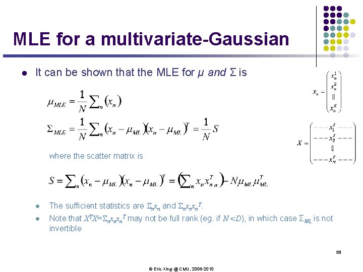
MLE for a multivariate-Gaussian l It can be shown that the MLE for µ and Σ is where the scatter matrix is l The sufficient statistics are Snxn and Snxnxn. T. l Note that XTX=Snxnxn. T may not be full rank (eg. if N <D), in which case ΣML is not invertible 58 © Eric Xing @ CMU, 2006 -2010

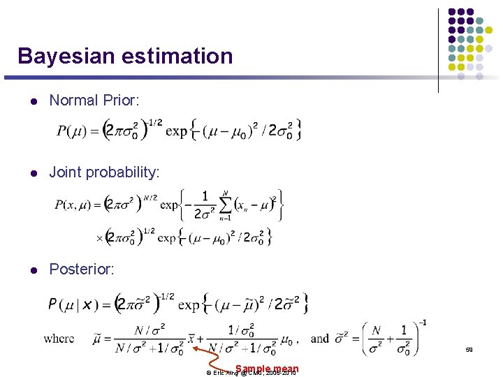
Bayesian estimation l Normal Prior: l Joint probability: l Posterior: 59 mean © Eric Xing. Sample @ CMU, 2006 -2010

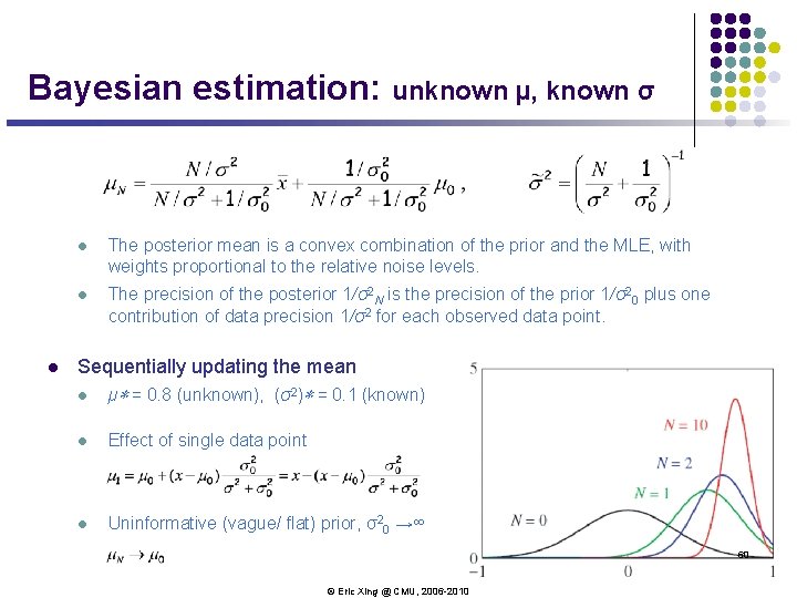
Bayesian estimation: unknown µ, known σ l l The posterior mean is a convex combination of the prior and the MLE, with weights proportional to the relative noise levels. l The precision of the posterior 1/σ2 N is the precision of the prior 1/σ20 plus one contribution of data precision 1/σ2 for each observed data point. Sequentially updating the mean l µ∗ = 0. 8 (unknown), (σ2)∗ = 0. 1 (known) l Effect of single data point l Uninformative (vague/ flat) prior, σ20 →∞ 60 © Eric Xing @ CMU, 2006 -2010