Support Vector Machines SVMs Section 5 11 Duda

Support Vector Machines (SVMs) Section 5. 11 (Duda et al. ) CS 479/679 Pattern Recognition Dr. George Bebis

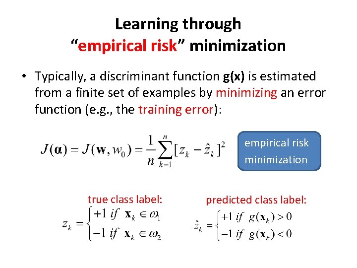
Learning through “empirical risk” minimization • Typically, a discriminant function g(x) is estimated from a finite set of examples by minimizing an error function (e. g. , the training error): empirical risk minimization true class label: predicted class label:

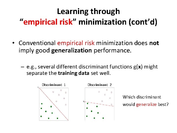
Learning through “empirical risk” minimization (cont’d) • Conventional empirical risk minimization does not imply good generalization performance. – e. g. , several different discriminant functions g(x) might separate the training data set well. Discriminant 1 Discriminant 2 Which discriminant would generalize best?

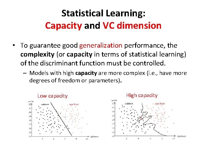
Statistical Learning: Capacity and VC dimension • To guarantee good generalization performance, the complexity (or capacity in terms of statistical learning) of the discriminant function must be controlled. – Models with high capacity are more complex (i. e. , have more degrees of freedom or parameters). Low capacity High capacity

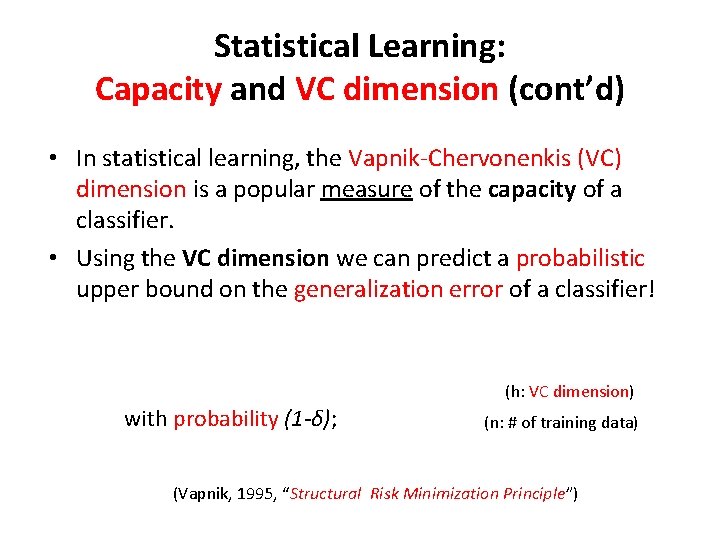
Statistical Learning: Capacity and VC dimension (cont’d) • In statistical learning, the Vapnik-Chervonenkis (VC) dimension is a popular measure of the capacity of a classifier. • Using the VC dimension we can predict a probabilistic upper bound on the generalization error of a classifier! (h: VC dimension) with probability (1 -δ); (n: # of training data) (Vapnik, 1995, “Structural Risk Minimization Principle”)

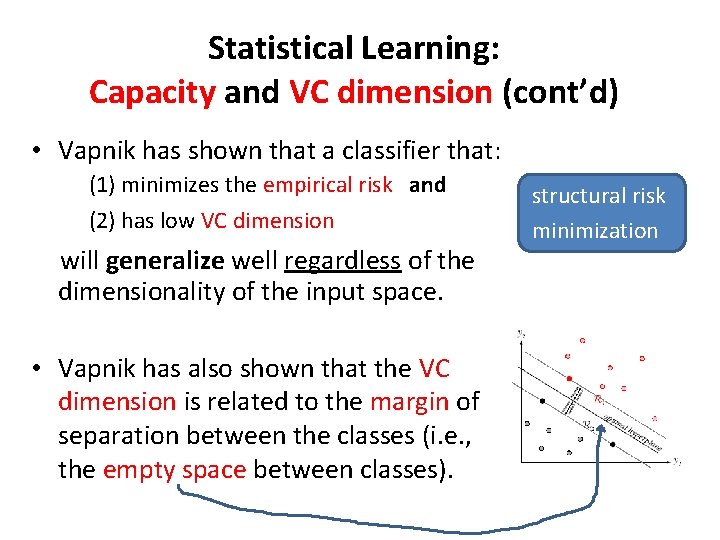
Statistical Learning: Capacity and VC dimension (cont’d) • Vapnik has shown that a classifier that: (1) minimizes the empirical risk and (2) has low VC dimension will generalize well regardless of the dimensionality of the input space. • Vapnik has also shown that the VC dimension is related to the margin of separation between the classes (i. e. , the empty space between classes). structural risk minimization

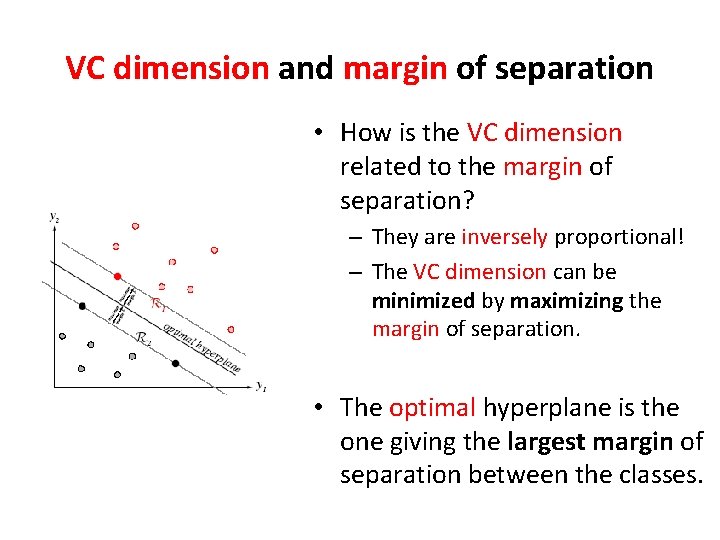
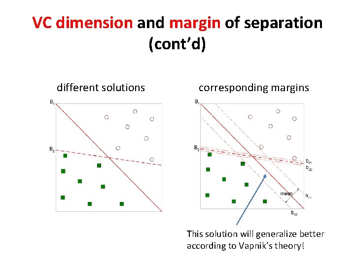
VC dimension and margin of separation • How is the VC dimension related to the margin of separation? – They are inversely proportional! – The VC dimension can be minimized by maximizing the margin of separation. • The optimal hyperplane is the one giving the largest margin of separation between the classes.

VC dimension and margin of separation (cont’d) different solutions corresponding margins This solution will generalize better according to Vapnik’s theory!

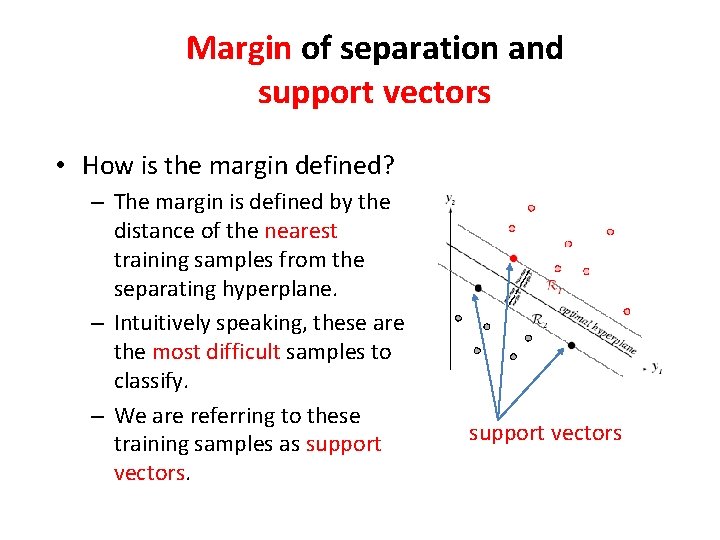
Margin of separation and support vectors • How is the margin defined? – The margin is defined by the distance of the nearest training samples from the separating hyperplane. – Intuitively speaking, these are the most difficult samples to classify. – We are referring to these training samples as support vectors

SVM Overview • Primarily a two-classifier - can be extended to multiple classes. • It performs structural risk minimization to achieve good generalization performance. • “Training” involves solving a quadratic programming problem with linear constraints. – Non-iterative, unlike Gradient Descent and Newton’s method which are iterative optimization algorithms!

Linear and Non-Linear SVMs • We will discuss the following three cases: – Linear SVM classifier assuming linearly separable data – Linear SVM classifier assuming non-linearly separable data (“soft margin” classifier) – Non-linear SVM classifier

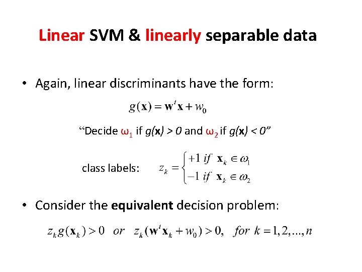
Linear SVM & linearly separable data • Again, linear discriminants have the form: “Decide ω1 if g(x) > 0 and ω2 if g(x) < 0” “ class labels: • Consider the equivalent decision problem:

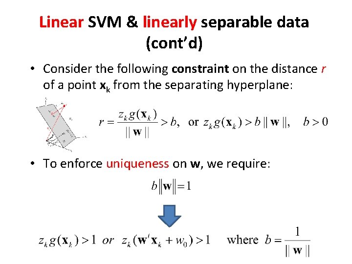
Linear SVM & linearly separable data (cont’d) • Consider the following constraint on the distance r of a point xk from the separating hyperplane: • To enforce uniqueness on w, we require:

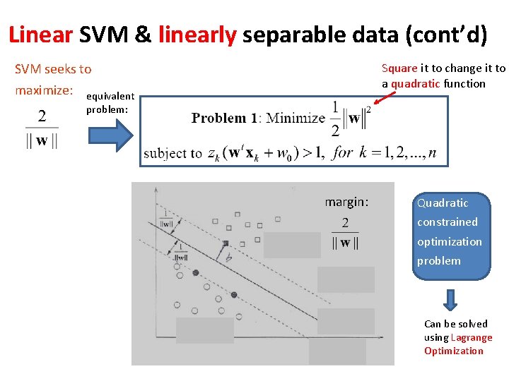
Linear SVM & linearly separable data (cont’d) SVM seeks to maximize: Square it to change it to a quadratic function equivalent problem: margin: Quadratic constrained optimization problem Can be solved using Lagrange Optimization

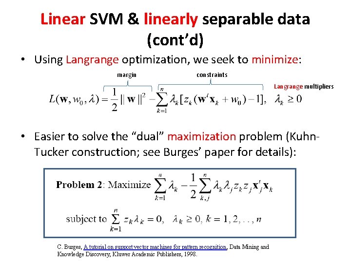
Linear SVM & linearly separable data (cont’d) • Using Langrange optimization, we seek to minimize: margin constraints Langrange multipliers • Easier to solve the “dual” maximization problem (Kuhn. Tucker construction; see Burges’ paper for details): C. Burges, A tutorial on support vector machines for pattern recognition, Data Mining and Knowledge Discovery, Kluwer Academic Publishers, 1998.

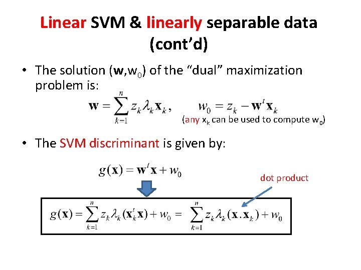
Linear SVM & linearly separable data (cont’d) • The solution (w, w 0) of the “dual” maximization problem is: (any xk can be used to compute w 0) • The SVM discriminant is given by: dot product

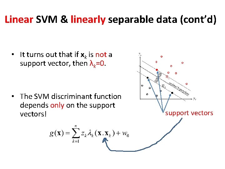
Linear SVM & linearly separable data (cont’d) • It turns out that if xk is not a support vector, then λk=0. • The SVM discriminant function depends only on the support vectors! support vectors

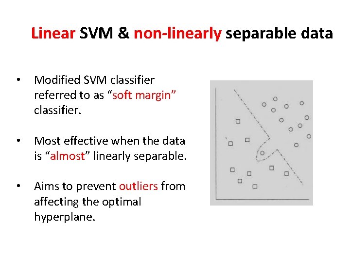
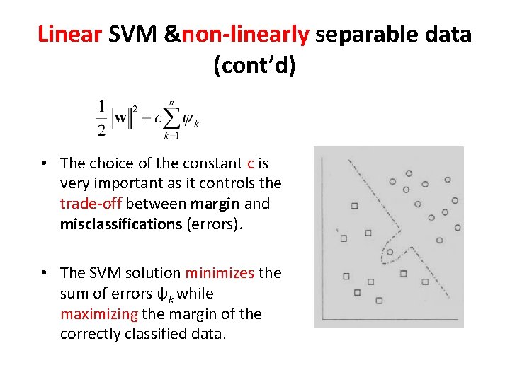
Linear SVM & non-linearly separable data • Modified SVM classifier referred to as “soft margin” classifier. • Most effective when the data is “almost” linearly separable. • Aims to prevent outliers from affecting the optimal hyperplane.

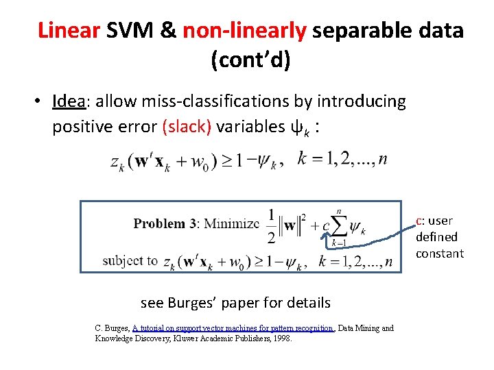
Linear SVM & non-linearly separable data (cont’d) • Idea: allow miss-classifications by introducing positive error (slack) variables ψk : c: user defined constant see Burges’ paper for details C. Burges, A tutorial on support vector machines for pattern recognition, Data Mining and Knowledge Discovery, Kluwer Academic Publishers, 1998.

Linear SVM &non-linearly separable data (cont’d) • The choice of the constant c is very important as it controls the trade-off between margin and misclassifications (errors). • The SVM solution minimizes the sum of errors ψk while maximizing the margin of the correctly classified data.

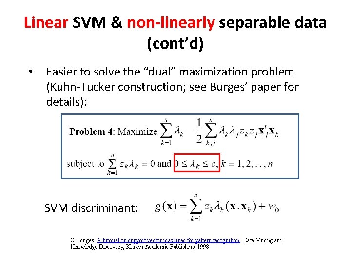
Linear SVM & non-linearly separable data (cont’d) • Easier to solve the “dual” maximization problem (Kuhn-Tucker construction; see Burges’ paper for details): SVM discriminant: C. Burges, A tutorial on support vector machines for pattern recognition, Data Mining and Knowledge Discovery, Kluwer Academic Publishers, 1998.

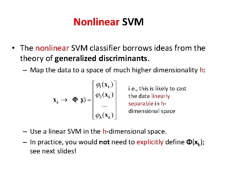
Nonlinear SVM • The nonlinear SVM classifier borrows ideas from theory of generalized discriminants. – Map the data to a space of much higher dimensionality h: i. e. , this is likely to cast the data linearly separable in hdimensional space – Use a linear SVM in the h-dimensional space. – In practice, you would not need to explicitly define Φ(xk); see next slides!

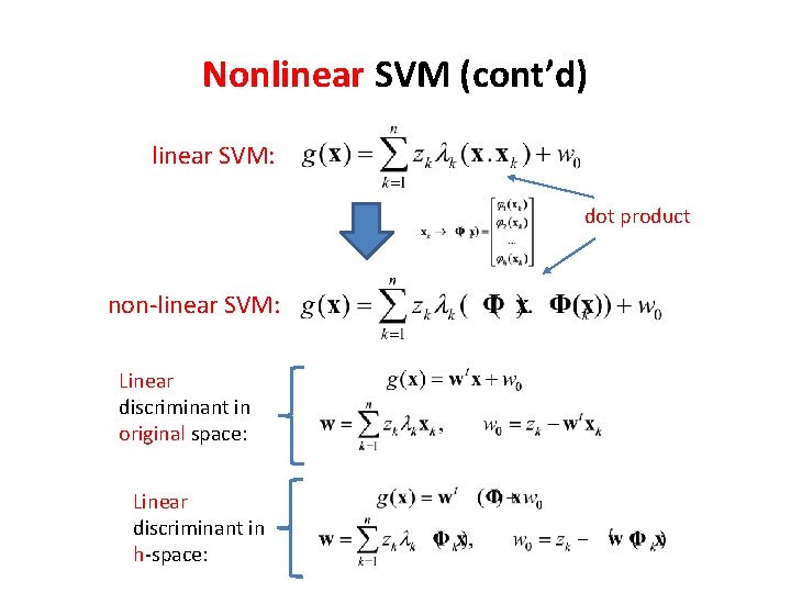
Nonlinear SVM (cont’d) linear SVM: dot product non-linear SVM: Linear discriminant in original space: Linear discriminant in h-space:

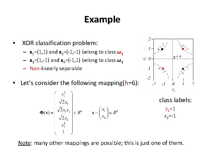
Example • XOR classification problem: – x 1=(1, 1) and x 2=(-1, -1) belong to class ω1 – x 3=(1, -1) and x 4=(-1, 1) belong to class ω2 – Non-linearly separable • Let’s consider the following mapping(h=6): class labels: z 1=1 z 2=-1 Note: many other mappings are possible; this is just one of them.

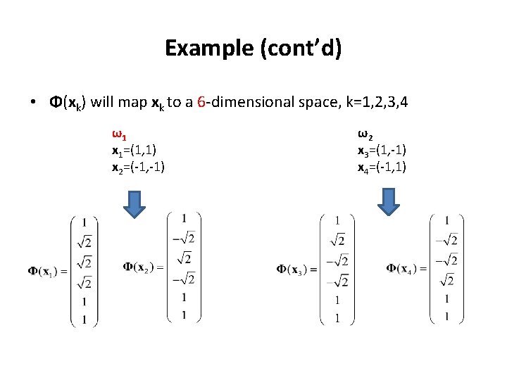
Example (cont’d) • Φ(xk) will map xk to a 6 -dimensional space, k=1, 2, 3, 4 ω1 x 1=(1, 1) x 2=(-1, -1) ω2 x 3=(1, -1) x 4=(-1, 1)

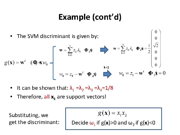
Example (cont’d) • The SVM discriminant is given by: k=1 • It can be shown that: λ 1 =λ 2 =λ 3 =λ 4=1/8 • Therefore, all xk are support vectors! Substituting, we get the discriminant: Decide ω1 if g(x)>0 and ω2 if g(x)<0

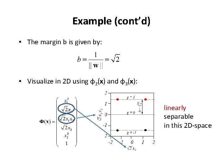
Example (cont’d) • The margin b is given by: • Visualize in 2 D using φ2(x) and φ3(x): linearly separable in this 2 D-space

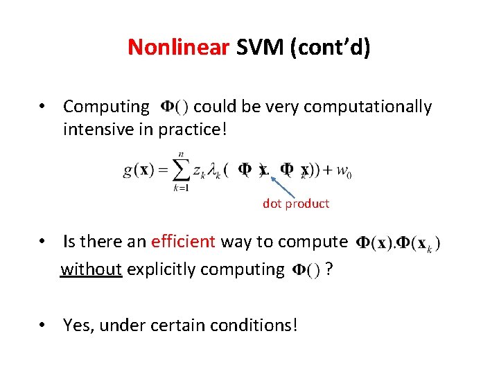
Nonlinear SVM (cont’d) • Computing could be very computationally intensive in practice! dot product • Is there an efficient way to compute without explicitly computing ? • Yes, under certain conditions!

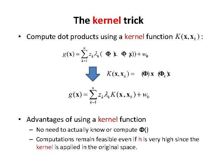
The kernel trick • Compute dot products using a kernel function • Advantages of using a kernel function – No need to actually know or compute Φ() – Computations remain feasible even if h is very high since the kernel is applied in the original space. :

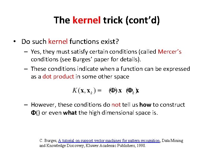
The kernel trick (cont’d) • Do such kernel functions exist? – Yes, they must satisfy certain conditions (called Mercer’s conditions (see Burges’ paper for details). – These conditions indicate when a function can be expressed as a dot product in some other space – However, these conditions do not tell us how to construct Φ() or even what the high dimensional space is. C. Burges, A tutorial on support vector machines for pattern recognition, Data Mining and Knowledge Discovery, Kluwer Academic Publishers, 1998.

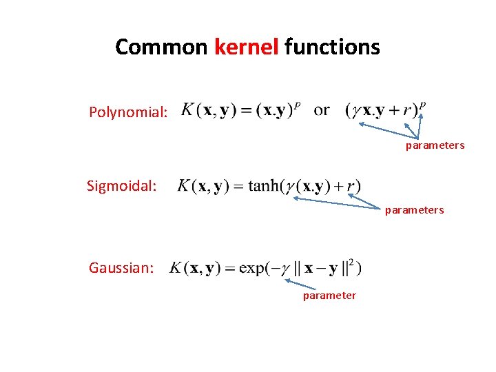
Common kernel functions Polynomial: parameters Sigmoidal: parameters Gaussian: parameter

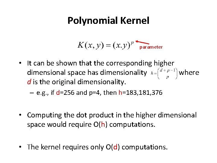
Polynomial Kernel parameter • It can be shown that the corresponding higher dimensional space has dimensionality where d is the original dimensionality. – e. g. , if d=256 and p=4, then h=183, 181, 376 • Computing the dot product in the higher dimensional space would require O(h) computations. • The kernel requires only O(d) computations.

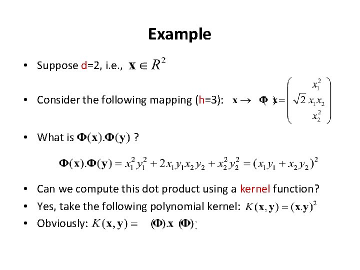
Example • Suppose d=2, i. e. , • Consider the following mapping (h=3): • What is ? • Can we compute this dot product using a kernel function? • Yes, take the following polynomial kernel: • Obviously:

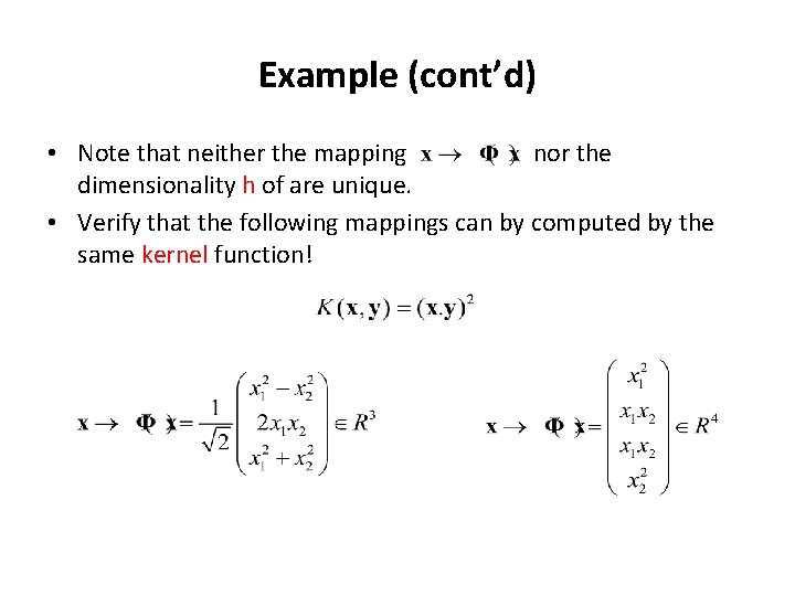
Example (cont’d) • Note that neither the mapping nor the dimensionality h of are unique. • Verify that the following mappings can by computed by the same kernel function!

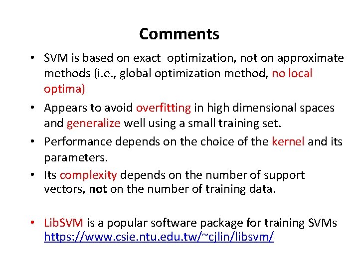
Comments • SVM is based on exact optimization, not on approximate methods (i. e. , global optimization method, no local optima) • Appears to avoid overfitting in high dimensional spaces and generalize well using a small training set. • Performance depends on the choice of the kernel and its parameters. • Its complexity depends on the number of support vectors, not on the number of training data. • Lib. SVM is a popular software package for training SVMs https: //www. csie. ntu. edu. tw/~cjlin/libsvm/

th 6 Quiz • When: Monday, May 3 rd at 2 pm – Closed book/notes – 10 minutes for answering the questions – 5 minutes for uploading your answers on Canvas (system will NOT accept any submissions after 2: 15 pm) – See “Course Overview” slides for details • What: Support Vector Machines