M Opper and G Sanguinetti Variational inference for

M. Opper and G. Sanguinetti Variational inference for Markov jump processes Guido Sanguinetti Joint work with Manfred Opper (T. U. Berlin)

M. Opper and G. Sanguinetti Talk plan • • • Markov jump processes in the life sciences Basics of jump processes Variational mean field Results Future extensions?

M. Opper and G. Sanguinetti Markov Jump Processes • Describe the dynamics of populations of interacting species • Changes in populations are discrete (birth/death) and happen at random times • Rates of births and deaths for a species depend on population levels for all species • Many examples: chemical kinetics, predator-prey models, telecoms, etc.

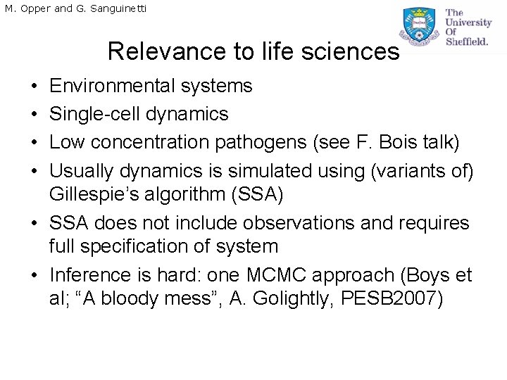
M. Opper and G. Sanguinetti Relevance to life sciences • • Environmental systems Single-cell dynamics Low concentration pathogens (see F. Bois talk) Usually dynamics is simulated using (variants of) Gillespie’s algorithm (SSA) • SSA does not include observations and requires full specification of system • Inference is hard: one MCMC approach (Boys et al; “A bloody mess”, A. Golightly, PESB 2007)

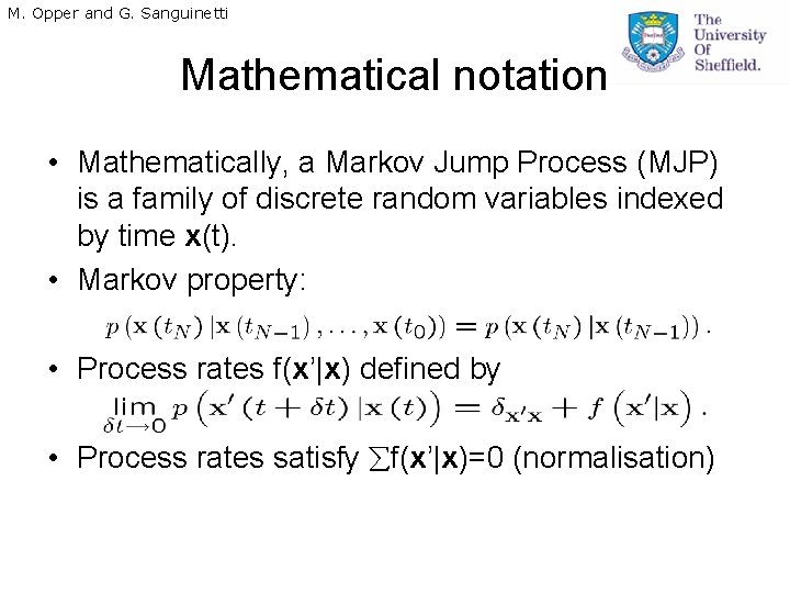
M. Opper and G. Sanguinetti Mathematical notation • Mathematically, a Markov Jump Process (MJP) is a family of discrete random variables indexed by time x(t). • Markov property: • Process rates f(x’|x) defined by • Process rates satisfy f(x’|x)=0 (normalisation)

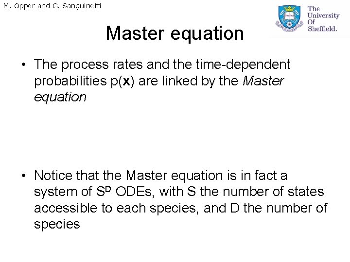
M. Opper and G. Sanguinetti Master equation • The process rates and the time-dependent probabilities p(x) are linked by the Master equation • Notice that the Master equation is in fact a system of SD ODEs, with S the number of states accessible to each species, and D the number of species

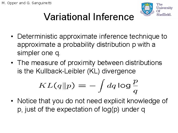
M. Opper and G. Sanguinetti Variational Inference • Deterministic approximate inference technique to approximate a probability distribution p with a simpler one q. • The measure of proximity between distributions is the Kullback-Leibler (KL) divergence • Notice that you do not need explicit knowledge of p, just of the expectation of log(p) under q

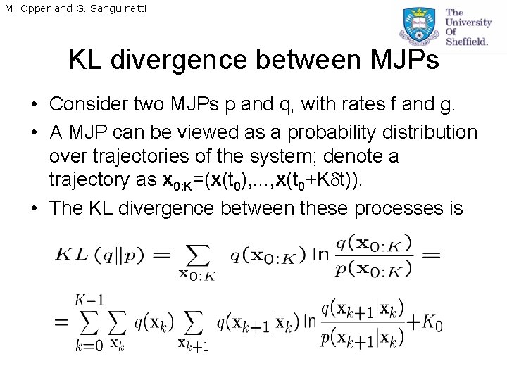
M. Opper and G. Sanguinetti KL divergence between MJPs • Consider two MJPs p and q, with rates f and g. • A MJP can be viewed as a probability distribution over trajectories of the system; denote a trajectory as x 0: K=(x(t 0), . . . , x(t 0+K t)). • The KL divergence between these processes is

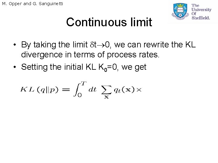
M. Opper and G. Sanguinetti Continuous limit • By taking the limit t 0, we can rewrite the KL divergence in terms of process rates. • Setting the initial KL K 0=0, we get

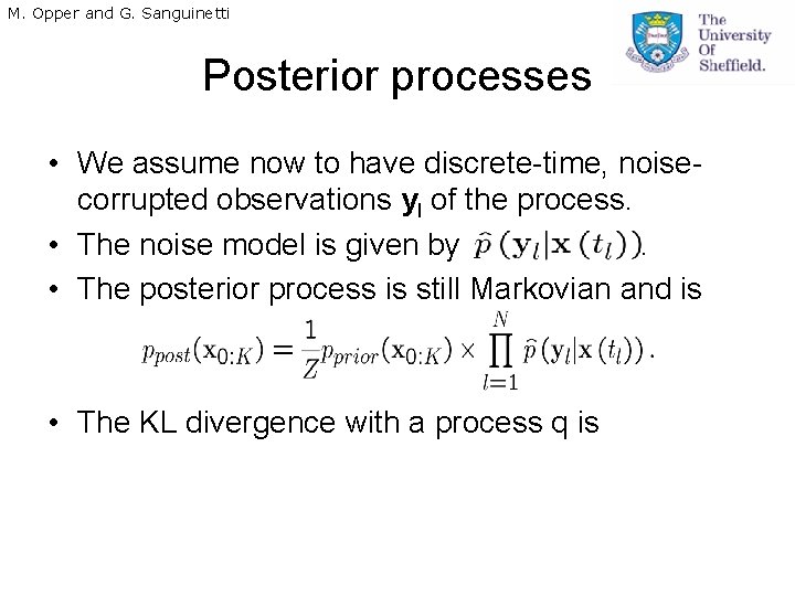
M. Opper and G. Sanguinetti Posterior processes • We assume now to have discrete-time, noisecorrupted observations yl of the process. • The noise model is given by. • The posterior process is still Markovian and is • The KL divergence with a process q is

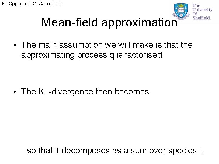
M. Opper and G. Sanguinetti Mean-field approximation • The main assumption we will make is that the approximating process q is factorised • The KL-divergence then becomes so that it decomposes as a sum over species i.

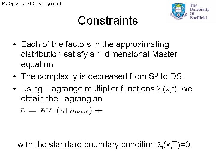
M. Opper and G. Sanguinetti Constraints • Each of the factors in the approximating distribution satisfy a 1 -dimensional Master equation. • The complexity is decreased from SD to DS. • Using Lagrange multiplier functions i(x, t), we obtain the Lagrangian with the standard boundary condition i(x, T)=0.

M. Opper and G. Sanguinetti Functional derivatives • To optimise the Lagrangian, we compute its functional derivatives

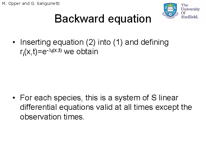
M. Opper and G. Sanguinetti Backward equation • Inserting equation (2) into (1) and defining ri(x, t)=e- i(x, t) we obtain • For each species, this is a system of S linear differential equations valid at all times except the observation times.

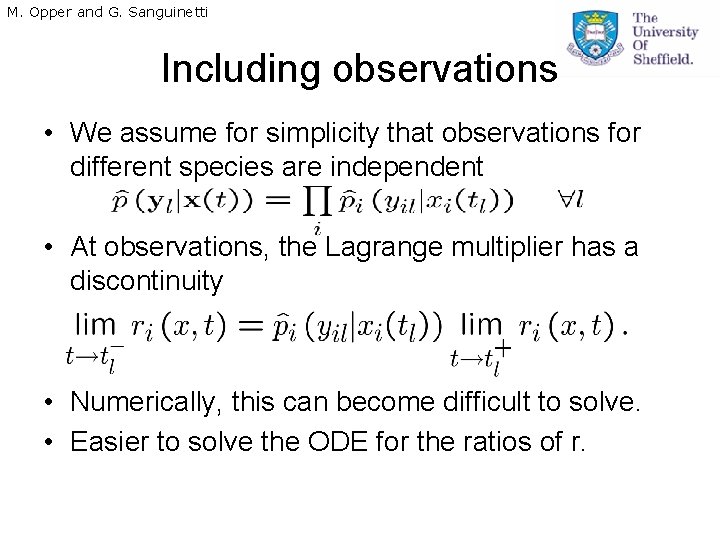
M. Opper and G. Sanguinetti Including observations • We assume for simplicity that observations for different species are independent • At observations, the Lagrange multiplier has a discontinuity • Numerically, this can become difficult to solve. • Easier to solve the ODE for the ratios of r.

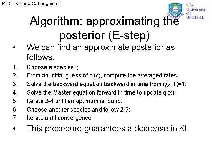
M. Opper and G. Sanguinetti Algorithm: approximating the posterior (E-step) • We can find an approximate posterior as follows: 1. 2. 3. 4. 5. 6. 7. Choose a species i; From an initial guess of qi(x), compute the averaged rates; Solve the backward equation backward in time from ri(x, T)=1; Solve the Master equation forward in time to update qi(x); Iterate 2 -4 until an optimum is found; Choose another species and follow 2 -5; Iterate until convergence. • This procedure guarantees a decrease in KL

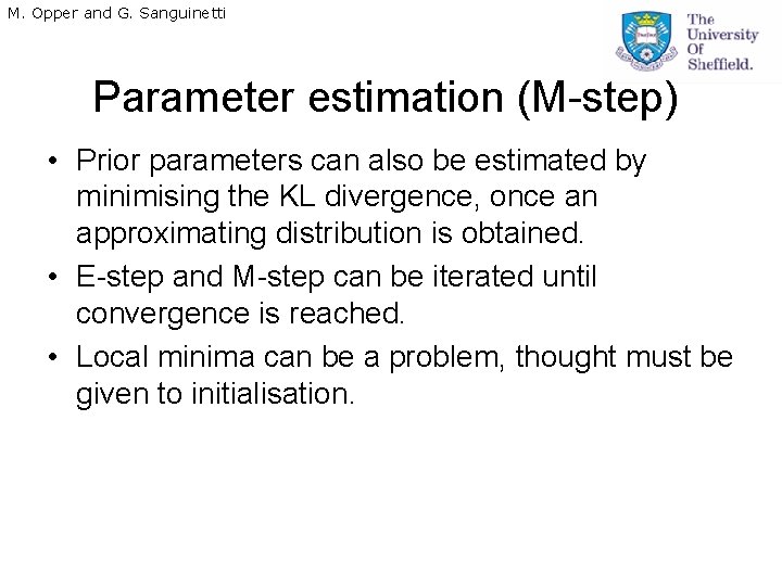
M. Opper and G. Sanguinetti Parameter estimation (M-step) • Prior parameters can also be estimated by minimising the KL divergence, once an approximating distribution is obtained. • E-step and M-step can be iterated until convergence is reached. • Local minima can be a problem, thought must be given to initialisation.

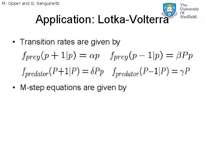
M. Opper and G. Sanguinetti Application: Lotka-Volterra • Transition rates are given by • M-step equations are given by

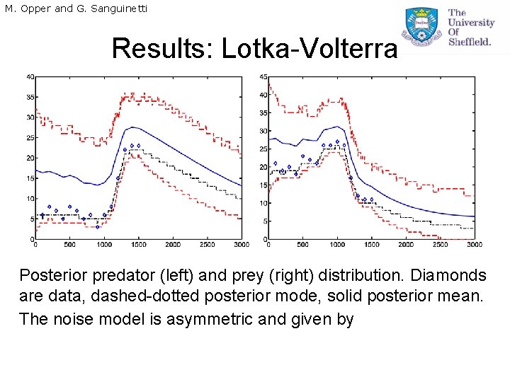
M. Opper and G. Sanguinetti Results: Lotka-Volterra Posterior predator (left) and prey (right) distribution. Diamonds are data, dashed-dotted posterior mode, solid posterior mean. The noise model is asymmetric and given by

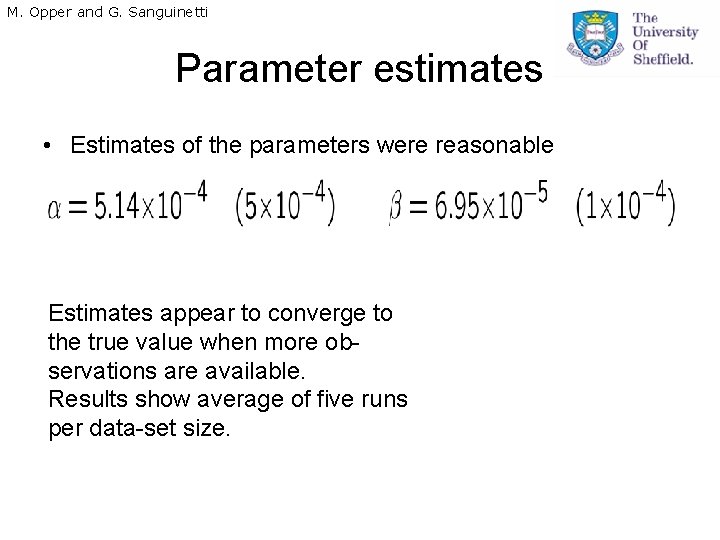
M. Opper and G. Sanguinetti Parameter estimates • Estimates of the parameters were reasonable Estimates appear to converge to the true value when more observations are available. Results show average of five runs per data-set size.

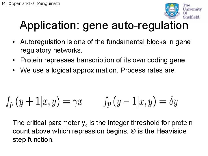
M. Opper and G. Sanguinetti Application: gene auto-regulation • Autoregulation is one of the fundamental blocks in gene regulatory networks. • Protein represses transcription of its own coding gene. • We use a logical approximation. Process rates are The critical parameter yc is the integer threshold for protein count above which repression begins. is the Heaviside step function.

M. Opper and G. Sanguinetti Parameter estimation • Fixed point equations for the parameters are obtained where is the posterior probability that the protein levels will be above the critical threshold (function of time).

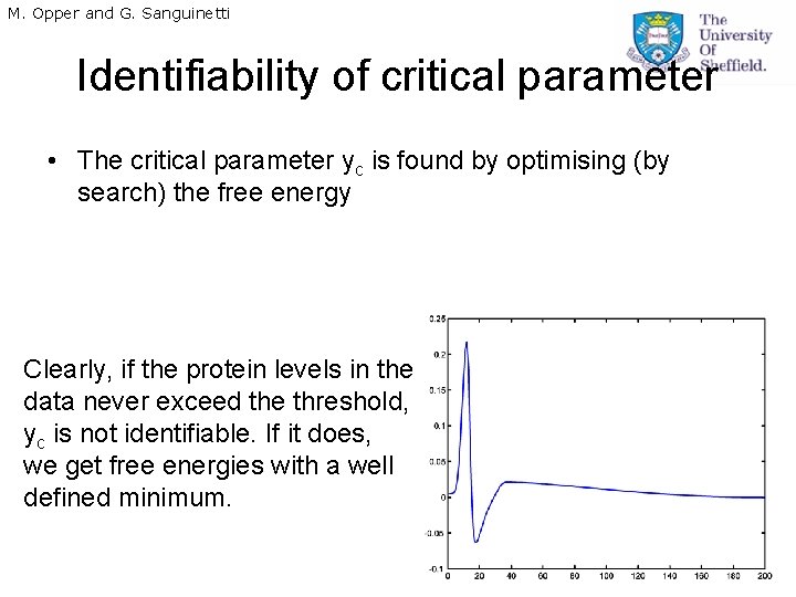
M. Opper and G. Sanguinetti Identifiability of critical parameter • The critical parameter yc is found by optimising (by search) the free energy Clearly, if the protein levels in the data never exceed the threshold, yc is not identifiable. If it does, we get free energies with a well defined minimum.

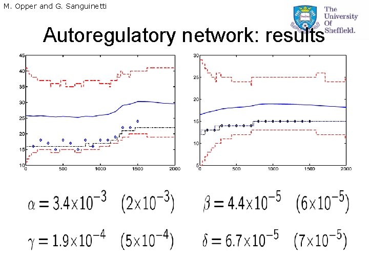
M. Opper and G. Sanguinetti Autoregulatory network: results

M. Opper and G. Sanguinetti Conclusions • Efficient framework for posterior inference and parameter estimation in MJPs. • Oustrips MCMC (Boys et al. ) by orders of magnitude. • Numerics are tricky and could be improved. • Issues swept under the carpet: regularisation, cut-off on number of states. • Readily extends to missing data.

M. Opper and G. Sanguinetti Future work • More complex, realistic networks. • Missing data. • Hybrid systems: one species has large numbers, so approximate as deterministic or diffusion. • Hybrid systems: particles also have a spatial dimension, and diffuse in the environment.