LowestCost Routing EE 122 Intro to Communication Networks

Lowest-Cost Routing EE 122: Intro to Communication Networks Fall 2010 (MW 4 -5: 30 in 101 Barker) Scott Shenker TAs: Sameer Agarwal, Sara Alspaugh, Igor Ganichev, Prayag Narula http: //inst. eecs. berkeley. edu/~ee 122/ Materials with thanks to Jennifer Rexford, Ion Stoica, Vern Paxson and other colleagues at Princeton and UC Berkeley 1

Announcements • Revision to lecture schedule – Advanced topics on routing • Revision to homework schedule – 3 a: get midterm questions right – 3 b: new topics • Changes to class structure – 5 minute “technology break” – Administrivia right after break – Group problem solving (when possible) o Sit next to smart people 2

Goals of Today’s Lecture • Routing overview: – Routing vs. forwarding – Routing topics • Link-state routing (Dijkstra’s algorithm) • Distance-vector routing (Bellman-Ford) 3

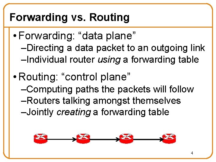
Forwarding vs. Routing • Forwarding: “data plane” –Directing a data packet to an outgoing link –Individual router using a forwarding table • Routing: “control plane” –Computing paths the packets will follow –Routers talking amongst themselves –Jointly creating a forwarding table 4

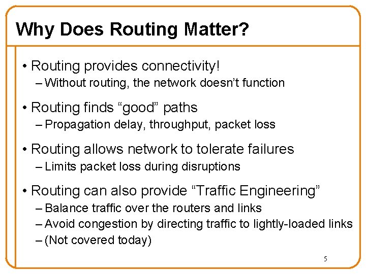
Why Does Routing Matter? • Routing provides connectivity! – Without routing, the network doesn’t function • Routing finds “good” paths – Propagation delay, throughput, packet loss • Routing allows network to tolerate failures – Limits packet loss during disruptions • Routing can also provide “Traffic Engineering” – Balance traffic over the routers and links – Avoid congestion by directing traffic to lightly-loaded links – (Not covered today) 5

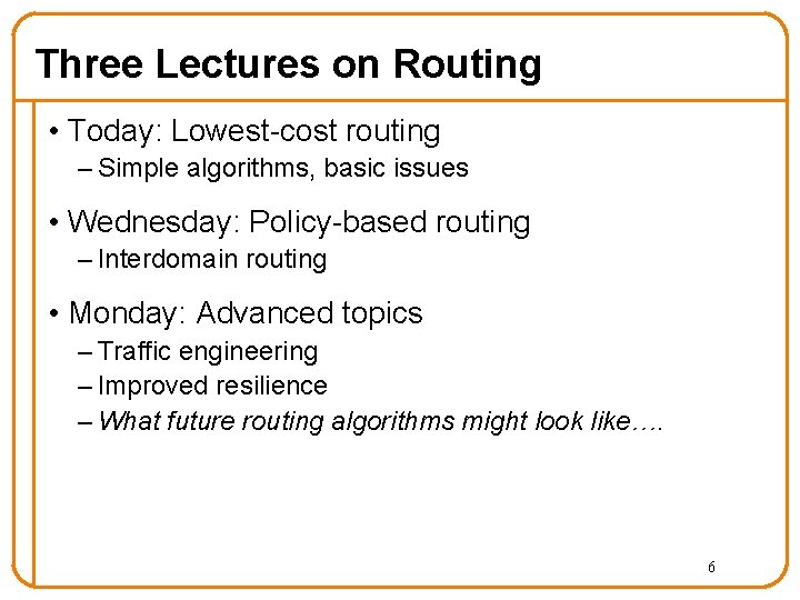
Three Lectures on Routing • Today: Lowest-cost routing – Simple algorithms, basic issues • Wednesday: Policy-based routing – Interdomain routing • Monday: Advanced topics – Traffic engineering – Improved resilience – What future routing algorithms might look like…. 6

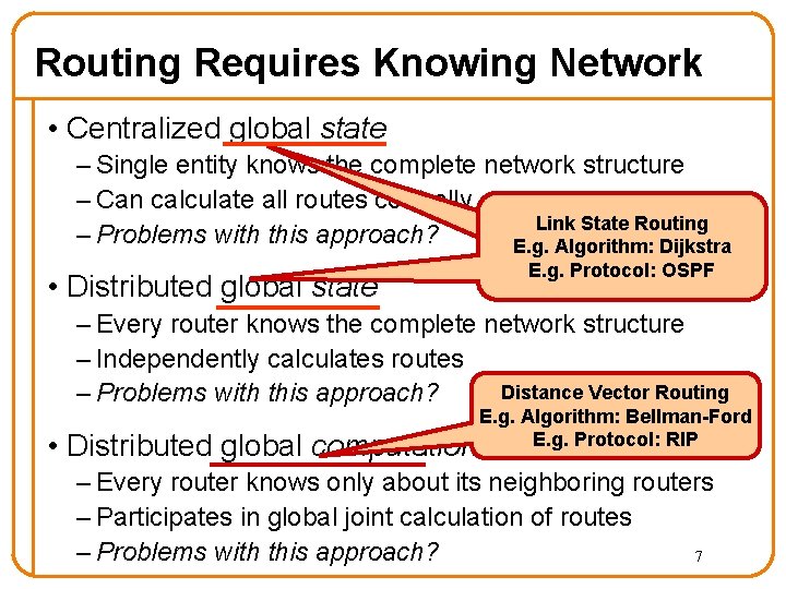
Routing Requires Knowing Network • Centralized global state – Single entity knows the complete network structure – Can calculate all routes centrally Link State Routing – Problems with this approach? E. g. Algorithm: Dijkstra • Distributed global state E. g. Protocol: OSPF – Every router knows the complete network structure – Independently calculates routes Distance Vector Routing – Problems with this approach? • Distributed global E. g. Algorithm: Bellman-Ford E. g. Protocol: RIP computation – Every router knows only about its neighboring routers – Participates in global joint calculation of routes – Problems with this approach? 7

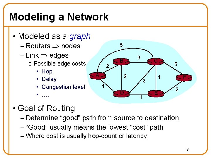
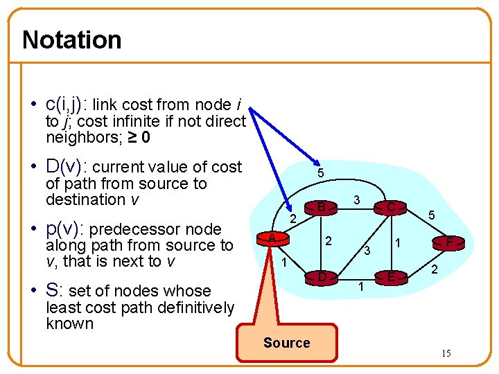
Modeling a Network • Modeled as a graph – Routers nodes – Link edges o Possible edge costs • Hop • Delay • Congestion level • …. 5 2 A 3 B 2 3 1 D C 1 5 F 1 E 2 • Goal of Routing – Determine “good” path from source to destination – “Good” usually means the lowest “cost” path – Where cost is usually hop-count or latency 8

From Model to Reality • In reality, attach prefixes to nodes • Calculate routing tables in terms of prefixes • But ignore this for now…. . – Just calculate paths between routers 9

Why Isn’t All Routing Lowest-Cost? • Lowest-cost routing assumes all nodes evaluate paths the same way – i. e. , use same “cost” metric • Interdomain routing: – Different domains care about different things – Can exercise general “policy” goals • Requires very different route computation – Talk about on Wednesday…. 10

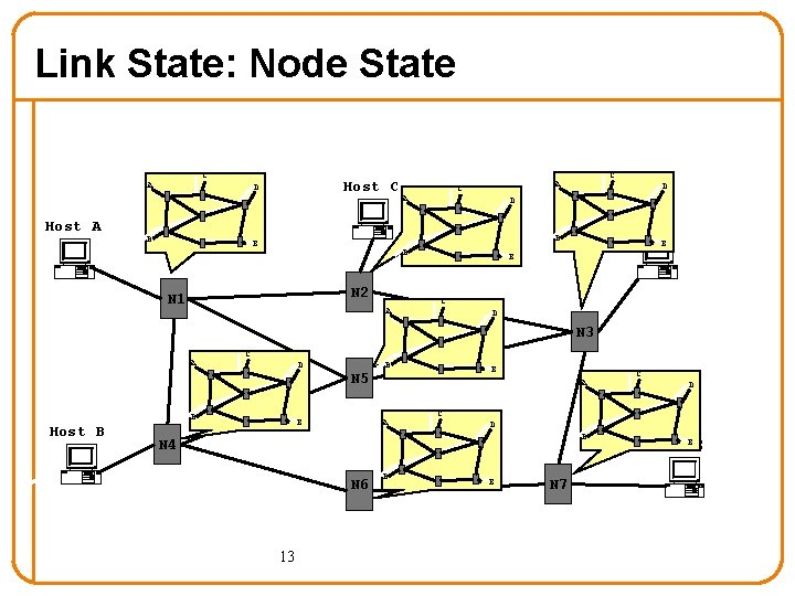
Link State Routing • Each router has complete network picture – Topology – Link costs • How does each router get the global state? – Each router reliably floods information about its neighbors to every other router (more later) • Each router independently calculates the shortest path from itself to every other router – Using, for example, Dijkstra’s Algorithm 11

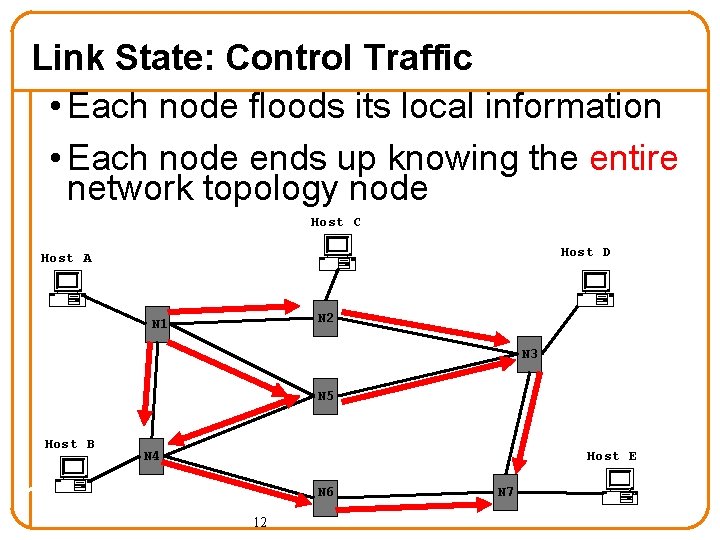
Link State: Control Traffic • Each node floods its local information • Each node ends up knowing the entire network topology node Host C Host D Host A N 2 N 1 N 3 N 5 Host B Host E N 4 N 6 12 N 7

Link State: Node State C A Host C D A C D D Host D B B E B N 2 N 1 A E E C D N 3 A C D B Host B N 5 E B E A A D B 13 B D C N 4 N 6 C E N 7 Host E E

Dijkstra’s Shortest Path Algorithm • INPUT: – Network topology (graph), with link costs • OUTPUT: – Least cost paths from one node to all other nodes – Produces “tree” of routes (why? ) 14

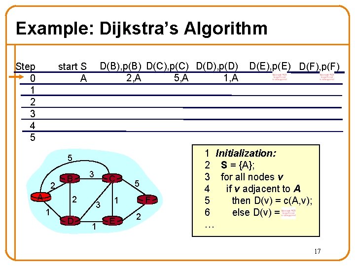
Notation • c(i, j): link cost from node i to j; cost infinite if not direct neighbors; ≥ 0 • D(v): current value of cost 5 of path from source to destination v • p(v): predecessor node along path from source to v, that is next to v 2 A B 2 1 D • S: set of nodes whose 3 C 3 1 5 F 1 E 2 least cost path definitively known Source 15

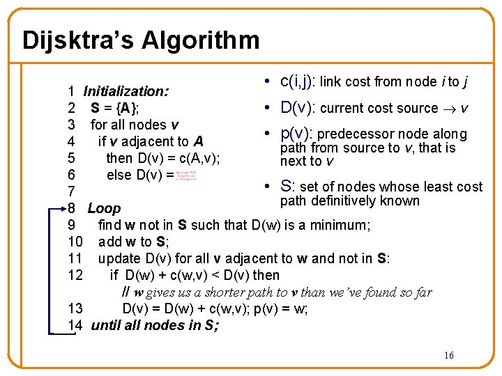
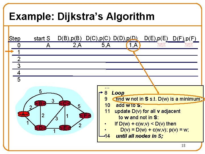
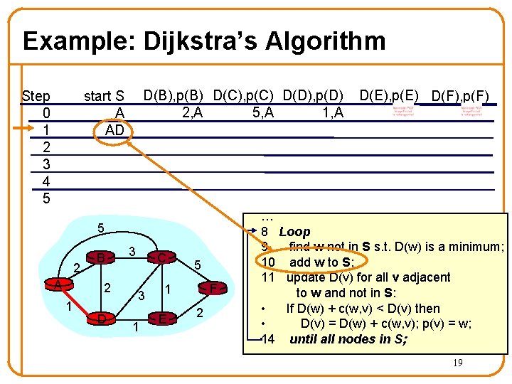
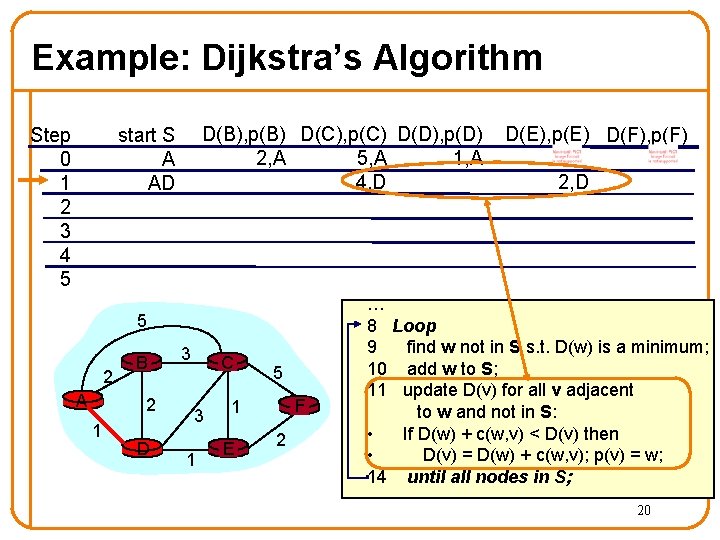
Dijsktra’s Algorithm • c(i, j): link cost from node i to j 1 Initialization: • D(v): current cost source v 2 S = {A}; 3 for all nodes v • p(v): predecessor node along 4 if v adjacent to A path from source to v, that is 5 then D(v) = c(A, v); next to v 6 else D(v) = ; • S: set of nodes whose least cost 7 path definitively known 8 Loop 9 find w not in S such that D(w) is a minimum; 10 add w to S; 11 update D(v) for all v adjacent to w and not in S: 12 if D(w) + c(w, v) < D(v) then // w gives us a shorter path to v than we’ve found so far 13 D(v) = D(w) + c(w, v); p(v) = w; 14 until all nodes in S; 16

Example: Dijkstra’s Algorithm Step 0 1 2 3 4 5 D(B), p(B) D(C), p(C) D(D), p(D) 2, A 1, A 5, A start S A 5 2 A B 2 1 D 3 C 3 1 5 F 1 E 2 D(E), p(E) D(F), p(F) 1 Initialization: 2 S = {A}; 3 for all nodes v 4 if v adjacent to A 5 then D(v) = c(A, v); 6 else D(v) = ; … 17

Example: Dijkstra’s Algorithm Step 0 1 2 3 4 5 D(B), p(B) D(C), p(C) D(D), p(D) 2, A 1, A 5, A start S A 5 2 A B 2 1 D 3 C 3 1 5 F 1 E 2 D(E), p(E) D(F), p(F) … 8 Loop 9 find w not in S s. t. D(w) is a minimum; 10 add w to S; 11 update D(v) for all v adjacent to w and not in S: • If D(w) + c(w, v) < D(v) then • D(v) = D(w) + c(w, v); p(v) = w; 14 until all nodes in S; 18

Example: Dijkstra’s Algorithm Step 0 1 2 3 4 5 D(B), p(B) D(C), p(C) D(D), p(D) 2, A 1, A 5, A start S A AD 5 2 A B 2 1 D 3 C 3 1 5 F 1 E 2 D(E), p(E) D(F), p(F) … 8 Loop 9 find w not in S s. t. D(w) is a minimum; 10 add w to S; 11 update D(v) for all v adjacent to w and not in S: • If D(w) + c(w, v) < D(v) then • D(v) = D(w) + c(w, v); p(v) = w; 14 until all nodes in S; 19

Example: Dijkstra’s Algorithm Step 0 1 2 3 4 5 D(B), p(B) D(C), p(C) D(D), p(D) 2, A 1, A 5, A 4, D start S A AD 5 2 A B 2 1 D 3 C 3 1 5 F 1 E 2 D(E), p(E) D(F), p(F) 2, D … 8 Loop 9 find w not in S s. t. D(w) is a minimum; 10 add w to S; 11 update D(v) for all v adjacent to w and not in S: • If D(w) + c(w, v) < D(v) then • D(v) = D(w) + c(w, v); p(v) = w; 14 until all nodes in S; 20

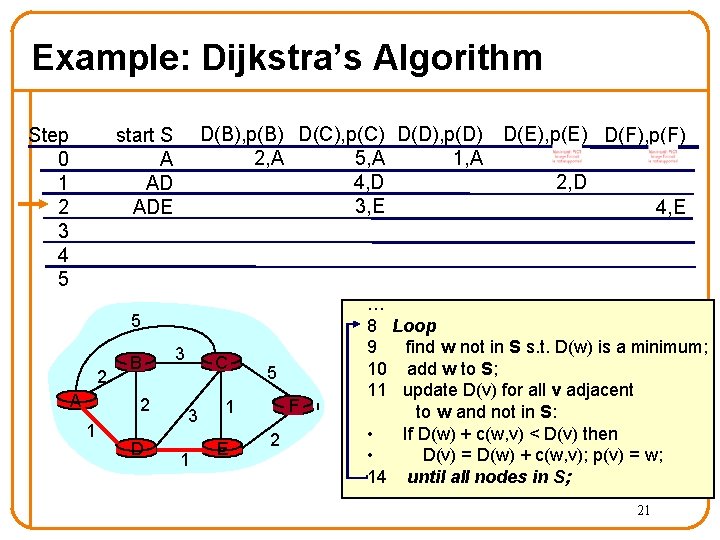
Example: Dijkstra’s Algorithm Step 0 1 2 3 4 5 D(B), p(B) D(C), p(C) D(D), p(D) D(E), p(E) D(F), p(F) 2, A 1, A 5, A 4, D 2, D 3, E 4, E start S A AD ADE 5 2 A B 2 1 D 3 C 3 1 5 F 1 E 2 … 8 Loop 9 find w not in S s. t. D(w) is a minimum; 10 add w to S; 11 update D(v) for all v adjacent to w and not in S: • If D(w) + c(w, v) < D(v) then • D(v) = D(w) + c(w, v); p(v) = w; 14 until all nodes in S; 21

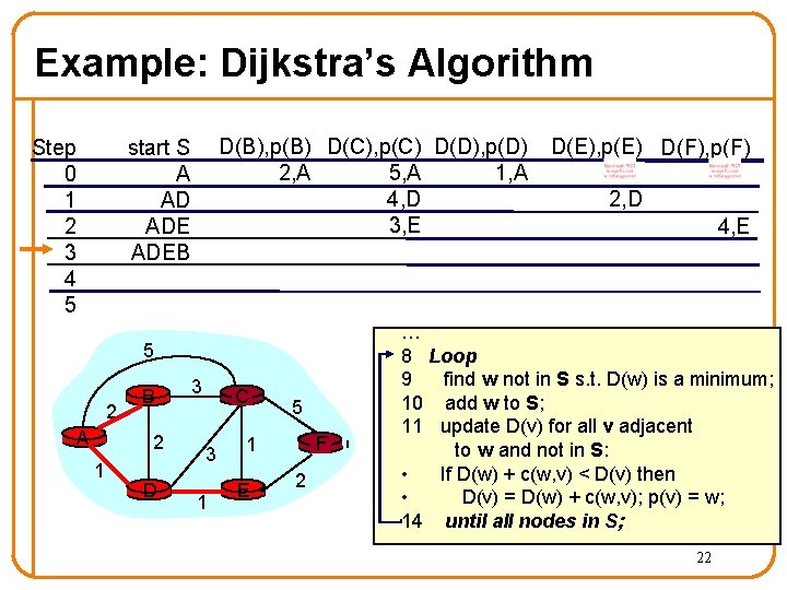
Example: Dijkstra’s Algorithm Step 0 1 2 3 4 5 D(B), p(B) D(C), p(C) D(D), p(D) 2, A 1, A 5, A 4, D 3, E start S A AD ADEB 5 2 A B 2 1 D 3 C 3 1 5 F 1 E 2 D(E), p(E) D(F), p(F) 2, D 4, E … 8 Loop 9 find w not in S s. t. D(w) is a minimum; 10 add w to S; 11 update D(v) for all v adjacent to w and not in S: • If D(w) + c(w, v) < D(v) then • D(v) = D(w) + c(w, v); p(v) = w; 14 until all nodes in S; 22

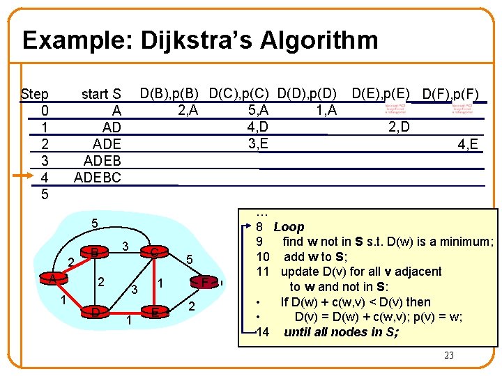
Example: Dijkstra’s Algorithm Step 0 1 2 3 4 5 D(B), p(B) D(C), p(C) D(D), p(D) 2, A 1, A 5, A 4, D 3, E start S A AD ADEBC 5 2 A B 2 1 D 3 C 3 1 5 F 1 E 2 D(E), p(E) D(F), p(F) 2, D 4, E … 8 Loop 9 find w not in S s. t. D(w) is a minimum; 10 add w to S; 11 update D(v) for all v adjacent to w and not in S: • If D(w) + c(w, v) < D(v) then • D(v) = D(w) + c(w, v); p(v) = w; 14 until all nodes in S; 23

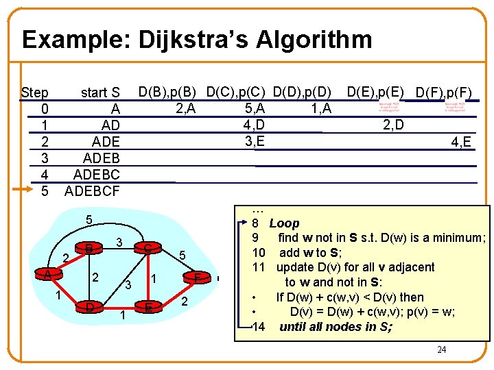
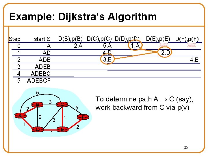
Example: Dijkstra’s Algorithm Step 0 1 2 3 4 5 D(B), p(B) D(C), p(C) D(D), p(D) 2, A 1, A 5, A 4, D 3, E start S A AD ADEBCF 5 2 A B 2 1 D 3 C 3 1 5 F 1 E 2 D(E), p(E) D(F), p(F) 2, D 4, E … 8 Loop 9 find w not in S s. t. D(w) is a minimum; 10 add w to S; 11 update D(v) for all v adjacent to w and not in S: • If D(w) + c(w, v) < D(v) then • D(v) = D(w) + c(w, v); p(v) = w; 14 until all nodes in S; 24

Example: Dijkstra’s Algorithm Step 0 1 2 3 4 5 D(B), p(B) D(C), p(C) D(D), p(D) 2, A 1, A 5, A 4, D 3, E start S A AD ADEBCF 5 2 A B 2 1 D 3 C 3 1 2, D 4, E To determine path A C (say), work backward from C via p(v) 5 F 1 E D(E), p(E) D(F), p(F) 2 25

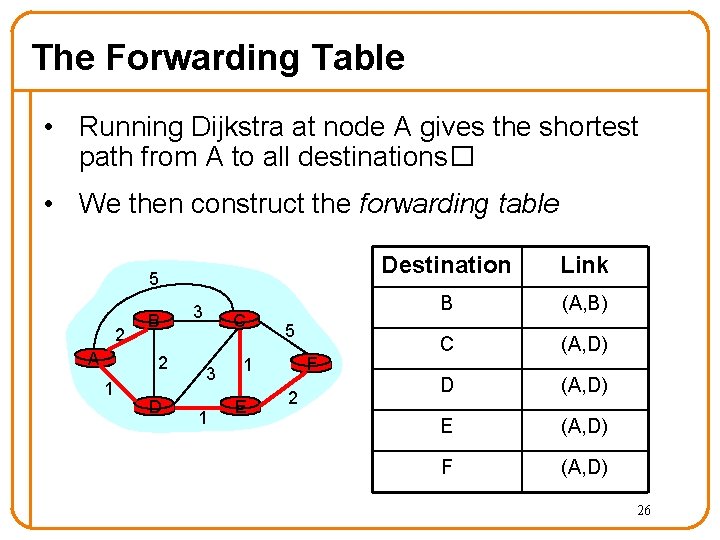
The Forwarding Table • Running Dijkstra at node A gives the shortest path from A to all destinations� • We then construct the forwarding table 5 2 A B 2 1 D 3 C 3 1 5 F 1 E 2 Destination Link B (A, B) C (A, D) D (A, D) E (A, D) F (A, D) 26

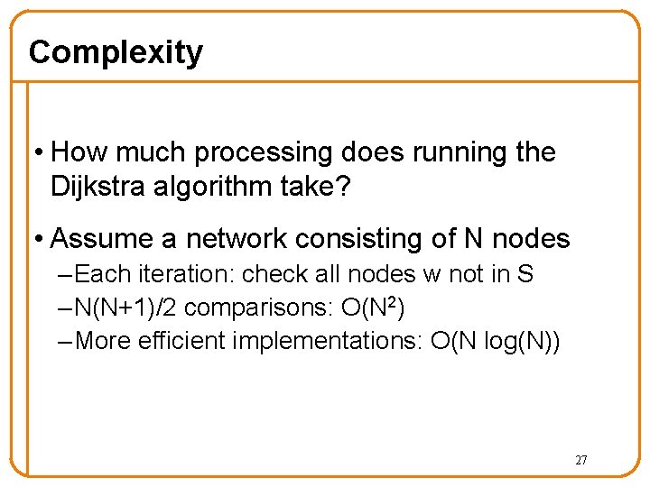
Complexity • How much processing does running the Dijkstra algorithm take? • Assume a network consisting of N nodes – Each iteration: check all nodes w not in S – N(N+1)/2 comparisons: O(N 2) – More efficient implementations: O(N log(N)) 27

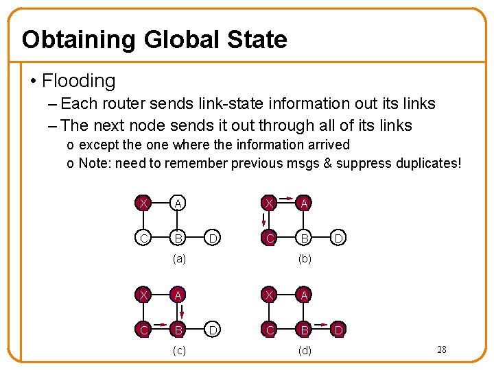
Obtaining Global State • Flooding – Each router sends link-state information out its links – The next node sends it out through all of its links o except the one where the information arrived o Note: need to remember previous msgs & suppress duplicates! X A C B D X A C B (a) X A C B (c) D (b) D X A C B (d) D 28

Flooding the Link State • Reliable flooding – Ensure all nodes receive link-state information – Ensure all nodes use the latest version • Challenges – Packet loss – Out-of-order arrival • Solutions – Acknowledgments and retransmissions – Sequence numbers 29

When to Initiate Flooding • Topology change – Link or node failure – Link or node recovery • Configuration change – Link cost change – Potential problems with making cost dynamic! • Periodically – Refresh the link-state information – Typically (say) 30 minutes – Corrects for possible corruption of the data 30

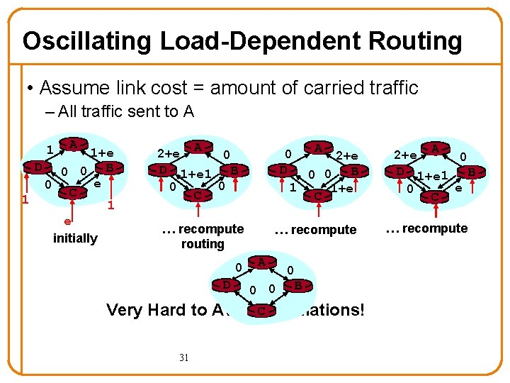
Oscillating Load-Dependent Routing • Assume link cost = amount of carried traffic – All traffic sent to A 1+e D 0 0 B e 0 C 1 1 e initially 2+e A 0 D 1+e 1 B 0 0 C A 0 2+e D 0 0 B 1 1+e C … recompute routing 0 D … recompute A 0 0 0 B Very Hard to Avoid. COscillations! 31 2+e A 0 D 1+e 1 B e 0 C … recompute

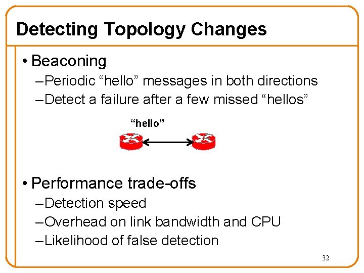
Detecting Topology Changes • Beaconing – Periodic “hello” messages in both directions – Detect a failure after a few missed “hellos” “hello” • Performance trade-offs – Detection speed – Overhead on link bandwidth and CPU – Likelihood of false detection 32

Convergence • Getting consistent routing information to all nodes – E. g. , all nodes having the same link-state database • Consistent forwarding after convergence – All nodes have the same link-state database – All nodes forward packets on shortest paths – The next router on the path forwards to the next hop 33

Convergence Delay • Time elapsed before every router has a consistent picture of the network • Sources of convergence delay – Detection latency – Flooding of link-state information – Recomputation of forwarding tables • Performance during convergence period – Lost packets due to blackholes and TTL expiry – Looping packets consuming resources – Out-of-order packets reaching the destination • Very bad for Vo. IP, online gaming, and video 34

Reducing Convergence Delay • Faster detection – Smaller hello timers – Link-layer technologies that can detect failures • Faster flooding – Flooding immediately – Sending link-state packets with high-priority • Faster computation – Faster processors on the routers – Incremental Dijkstra algorithm • Faster forwarding-table update – Data structures supporting incremental updates 35

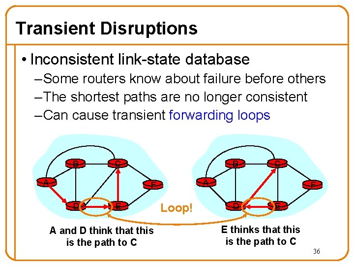
Transient Disruptions • Inconsistent link-state database – Some routers know about failure before others – The shortest paths are no longer consistent – Can cause transient forwarding loops B C A B A F D E A and D think that this is the path to C C Loop! F D E E thinks that this is the path to C 36

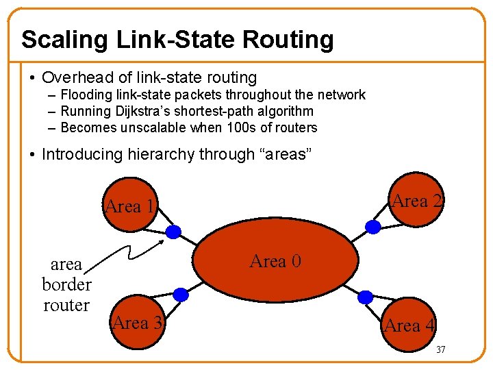
Scaling Link-State Routing • Overhead of link-state routing – Flooding link-state packets throughout the network – Running Dijkstra’s shortest-path algorithm – Becomes unscalable when 100 s of routers • Introducing hierarchy through “areas” Area 2 Area 1 area border router Area 0 Area 3 Area 4 37

Link-State Routing Is Conceptually Simple • Each router keeps track of its incident links – Link cost, and whether the link is up or down • Each router broadcasts the link state – To give every router a complete view of the graph • Each router runs Dijkstra’s algorithm – Compute shortest paths, then construct forwarding table • Example protocols – Open Shortest Path First (OSPF) – Intermediate System (IS-IS) • Challenges: scaling, transient disruptions – Any ideas for improvement? 38

Question • Why use different routing algorithms at L 2 and L 3? – Is Link-State “plug-and-play”? – Could we make it “plug-and-play? ” 39

5 Minute Break Questions Before We Proceed? 40

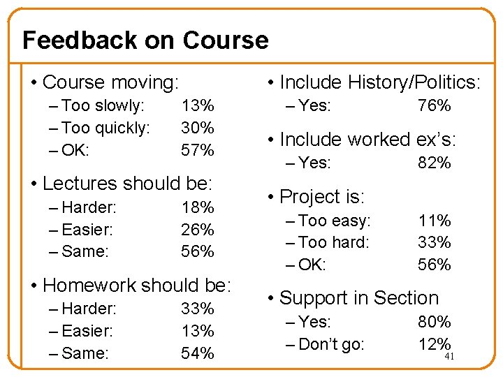
Feedback on Course • Course moving: – Too slowly: – Too quickly: – OK: • Include History/Politics: 13% 30% 57% • Lectures should be: – Harder: – Easier: – Same: 18% 26% 56% • Homework should be: – Harder: – Easier: – Same: 33% 13% 54% – Yes: 76% • Include worked ex’s: – Yes: 82% • Project is: – Too easy: – Too hard: – OK: 11% 33% 56% • Support in Section – Yes: – Don’t go: 80% 12% 41

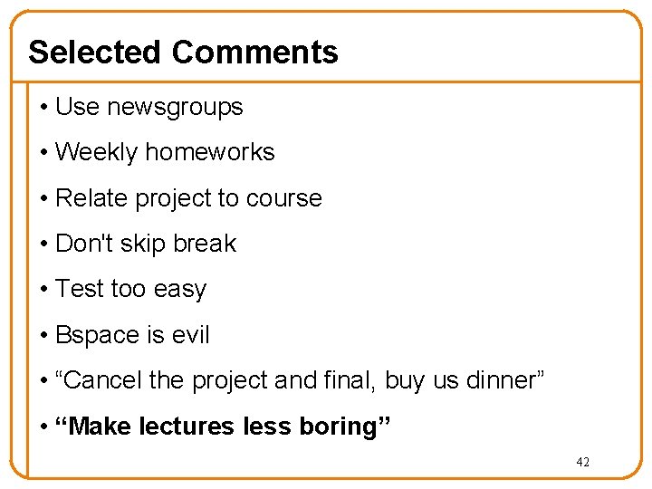
Selected Comments • Use newsgroups • Weekly homeworks • Relate project to course • Don't skip break • Test too easy • Bspace is evil • “Cancel the project and final, buy us dinner” • “Make lectures less boring” 42

More Scalable Routing Algorithms? • Avoid need for global state consistency • Just focus on computing routes • Distribute the computation, not the state…. 43

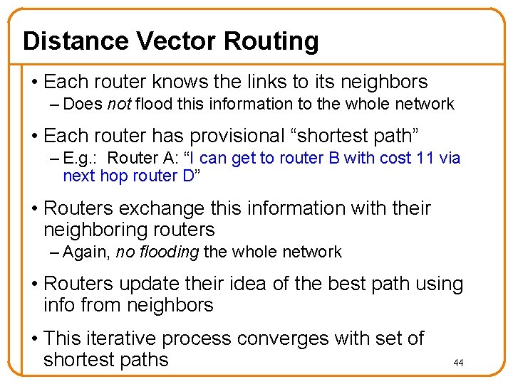
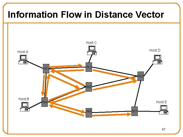
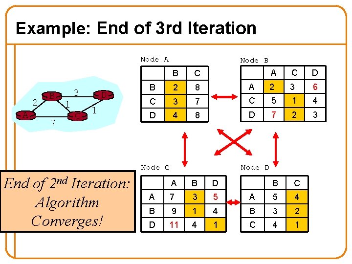
Distance Vector Routing • Each router knows the links to its neighbors – Does not flood this information to the whole network • Each router has provisional “shortest path” – E. g. : Router A: “I can get to router B with cost 11 via next hop router D” • Routers exchange this information with their neighboring routers – Again, no flooding the whole network • Routers update their idea of the best path using info from neighbors • This iterative process converges with set of shortest paths 44

Information Flow in Distance Vector Host C Host D Host A N 1 N 2 N 3 N 5 Host B Host E N 4 N 6 N 7 45

Information Flow in Distance Vector Host C Host D Host A N 1 N 2 N 3 N 5 Host B Host E N 4 N 6 N 7 46

Information Flow in Distance Vector Host C Host D Host A N 1 N 2 N 3 N 5 Host B Host E N 4 N 6 N 7 47

Why Is This Different From Flooding? 48

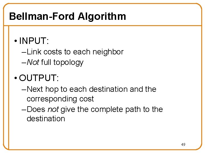
Bellman-Ford Algorithm • INPUT: – Link costs to each neighbor – Not full topology • OUTPUT: – Next hop to each destination and the corresponding cost – Does not give the complete path to the destination 49

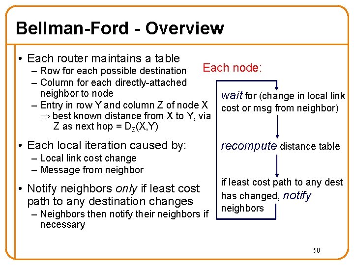
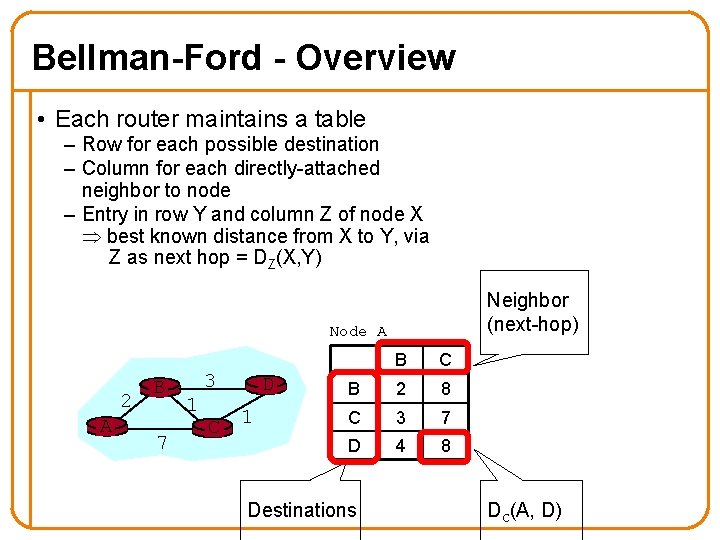
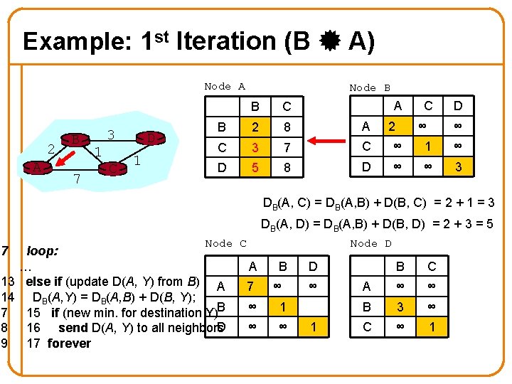
Bellman-Ford - Overview • Each router maintains a table Each node: – Row for each possible destination – Column for each directly-attached neighbor to node wait for (change in local link – Entry in row Y and column Z of node X cost or msg from neighbor) best known distance from X to Y, via Z as next hop = DZ(X, Y) • Each local iteration caused by: – Local link cost change – Message from neighbor • Notify neighbors only if least cost path to any destination changes – Neighbors then notify their neighbors if necessary recompute distance table if least cost path to any dest has changed, notify neighbors 50

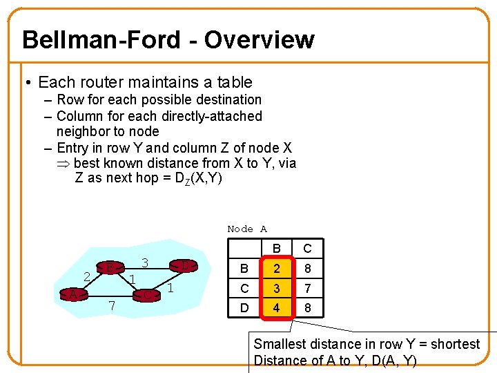
Bellman-Ford - Overview • Each router maintains a table – Row for each possible destination – Column for each directly-attached neighbor to node – Entry in row Y and column Z of node X best known distance from X to Y, via Z as next hop = DZ(X, Y) Neighbor (next-hop) Node A 2 A B 7 3 1 C D 1 B C B 2 8 C 3 7 D 4 8 Destinations DC(A, D)

Bellman-Ford - Overview • Each router maintains a table – Row for each possible destination – Column for each directly-attached neighbor to node – Entry in row Y and column Z of node X best known distance from X to Y, via Z as next hop = DZ(X, Y) Node A 2 A B 7 3 1 C D 1 B C B 2 8 C 3 7 D 4 8 Smallest distance in row Y = shortest Distance of A to Y, D(A, Y)

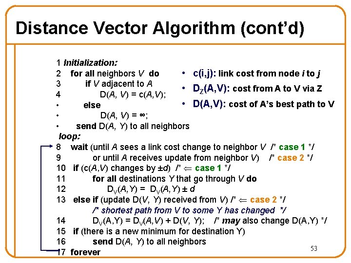
Distance Vector Algorithm (cont’d) 1 Initialization: 2 for all neighbors V do • c(i, j): link cost from node i to j 3 if V adjacent to A • DZ(A, V): cost from A to V via Z 4 D(A, V) = c(A, V); • D(A, V): cost of A’s best path to V • else • D(A, V) = ∞; • send D(A, Y) to all neighbors loop: 8 wait (until A sees a link cost change to neighbor V /* case 1 */ 9 or until A receives update from neighbor V) /* case 2 */ 10 if (c(A, V) changes by ±d) /* case 1 */ 11 for all destinations Y that go through V do 12 DV(A, Y) = DV(A, Y) ± d 13 else if (update D(V, Y) received from V) /* case 2 */ /* shortest path from V to some Y has changed */ 14 DV(A, Y) = DV(A, V) + D(V, Y); /* may also change D(A, Y) */ 15 if (there is a new minimum for destination Y) 16 send D(A, Y) to all neighbors 53 17 forever

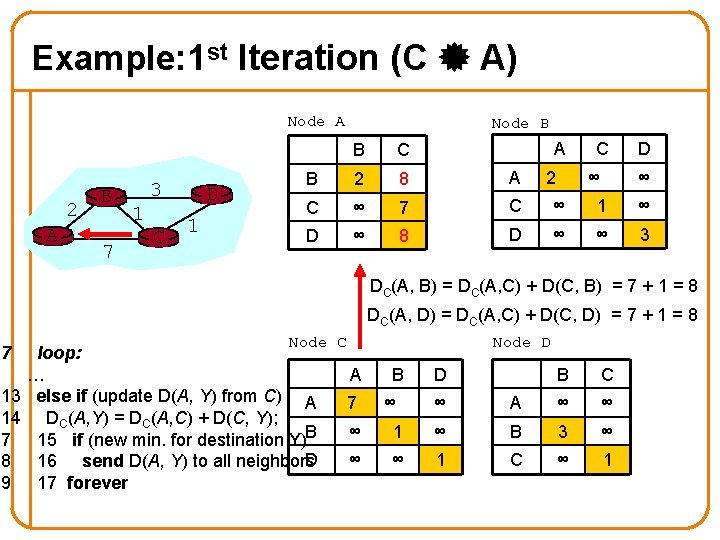
Example: 1 st Iteration (C A) Node A 2 A B 7 3 1 C D 1 Node B A C D B C B 2 8 A C ∞ 7 C ∞ 1 ∞ D ∞ 8 D ∞ ∞ 3 2 ∞ ∞ DC(A, B) = DC(A, C) + D(C, B) = 7 + 1 = 8 DC(A, D) = DC(A, C) + D(C, D) = 7 + 1 = 8 7 Node C loop: … 13 else if (update D(A, Y) from C) A 14 DC(A, Y) = DC(A, C) + D(C, Y); 7 15 if (new min. for destination Y)B D 8 16 send D(A, Y) to all neighbors 9 17 forever Node D A 7 B ∞ D B C ∞ A ∞ ∞ ∞ 1 ∞ B 3 ∞ ∞ ∞ 1 C ∞ 1

Example: 1 st Iteration (B A) Node A 2 A B 7 3 1 C D 1 Node B A C D B C B 2 8 A C 3 7 C ∞ 1 ∞ D 5 8 D ∞ ∞ 3 2 ∞ ∞ DB(A, C) = DB(A, B) + D(B, C) = 2 + 1 = 3 DB(A, D) = DB(A, B) + D(B, D) = 2 + 3 = 5 7 Node C loop: … 13 else if (update D(A, Y) from B) A 14 DB(A, Y) = DB(A, B) + D(B, Y); 7 15 if (new min. for destination Y)B D 8 16 send D(A, Y) to all neighbors 9 17 forever Node D A 7 B ∞ ∞ 1 ∞ ∞ D ∞ 1 B C A ∞ ∞ B 3 ∞ C ∞ 1

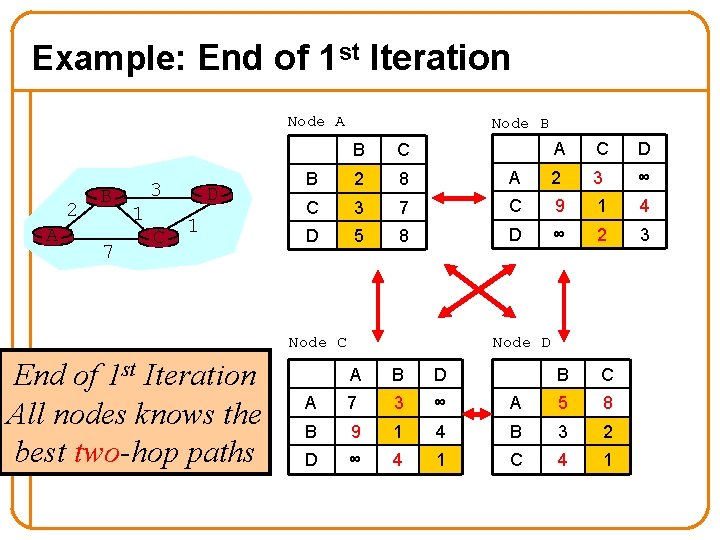
Example: End of 1 st Iteration Node A 2 A B 7 3 1 C D 1 Node B A C D A 2 3 ∞ 7 C 9 1 4 8 D ∞ 2 3 B C B 2 8 C 3 D 5 Node C End of 1 st Iteration All nodes knows the best two-hop paths Node D A B D A 7 3 ∞ A 5 8 B 9 1 4 B 3 2 D ∞ 4 1 C 4 1

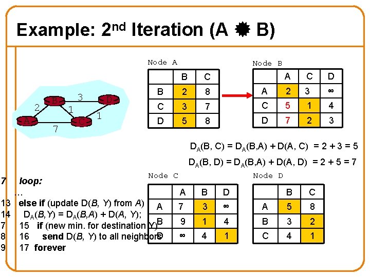
Example: 2 nd Iteration (A B) Node A 2 A B 7 3 1 C D 1 Node B A C D A 2 3 ∞ 7 C 5 1 4 8 D 7 2 3 B C B 2 8 C 3 D 5 DA(B, C) = DA(B, A) + D(A, C) = 2 + 3 = 5 DA(B, D) = DA(B, A) + D(A, D) = 2 + 5 = 7 7 Node C loop: … 13 else if (update D(B, Y) from A) A 14 DA(B, Y) = DA(B, A) + D(A, Y); 7 15 if (new min. for destination Y)B D 8 16 send D(B, Y) to all neighbors 9 17 forever Node D A B D B C 7 3 ∞ A 5 8 9 1 4 B 3 2 ∞ 4 1 C 4 1

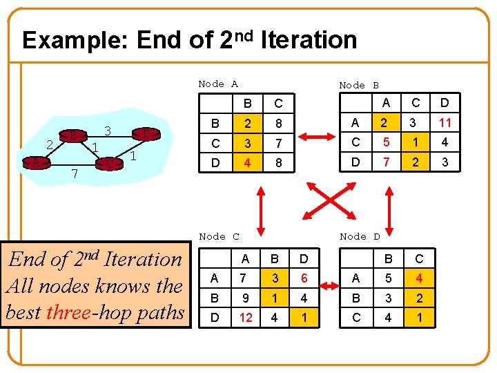
Example: End of 2 nd Iteration Node A 2 A B 7 3 1 C D 1 Node B A C D A 2 3 11 7 C 5 1 4 8 D 7 2 3 B C B 2 8 C 3 D 4 Node C End of 2 nd Iteration All nodes knows the best three-hop paths Node D A B D A 7 3 6 A 5 4 B 9 1 4 B 3 2 D 12 4 1 C 4 1

Example: End of 3 rd Iteration Node A 2 A B 7 3 1 C D 1 Node B A C D A 2 3 6 7 C 5 1 4 8 D 7 2 3 B C B 2 8 C 3 D 4 Node C End of 2 nd Iteration: Algorithm Converges! Node D A B D A 7 3 5 A 5 4 B 9 1 4 B 3 2 D 11 4 1 C 4 1

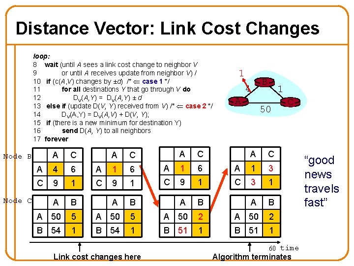
Distance Vector: Link Cost Changes loop: 8 wait (until A sees a link cost change to neighbor V 9 or until A receives update from neighbor V) / 10 if (c(A, V) changes by ±d) /* case 1 */ 11 for all destinations Y that go through V do 12 DV(A, Y) = DV(A, Y) ± d 13 else if (update D(V, Y) received from V) /* case 2 */ 14 DV(A, Y) = DV(A, V) + D(V, Y); 15 if (there is a new minimum for destination Y) 16 send D(A, Y) to all neighbors 17 forever A Node B Node C C A C 1 6 9 1 1 B 4 A 1 50 A C A 1 3 C 3 1 A 4 6 A 1 6 A C 9 1 C A B A B A 50 5 A 50 2 B 54 1 B 51 1 Link cost changes here C 60 time Algorithm terminates “good news travels fast”

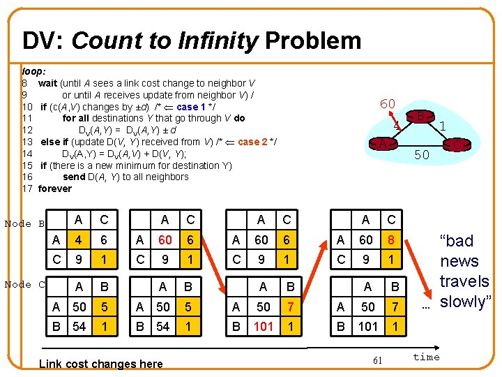
DV: Count to Infinity Problem loop: 8 wait (until A sees a link cost change to neighbor V 9 or until A receives update from neighbor V) / 10 if (c(A, V) changes by ±d) /* case 1 */ 11 for all destinations Y that go through V do 12 DV(A, Y) = DV(A, Y) ± d 13 else if (update D(V, Y) received from V) /* case 2 */ 14 DV(A, Y) = DV(A, V) + D(V, Y); 15 if (there is a new minimum for destination Y) 16 send D(A, Y) to all neighbors 17 forever A C A 4 6 A 60 6 C 9 1 A B A 50 5 A B 54 1 Node B Node C Link cost changes here 60 4 A A C A 60 6 C 9 1 A B 50 7 A B 101 1 1 50 A C A 60 8 C 9 1 A B 50 7 B 101 1 61 B C “bad news travels … slowly” time

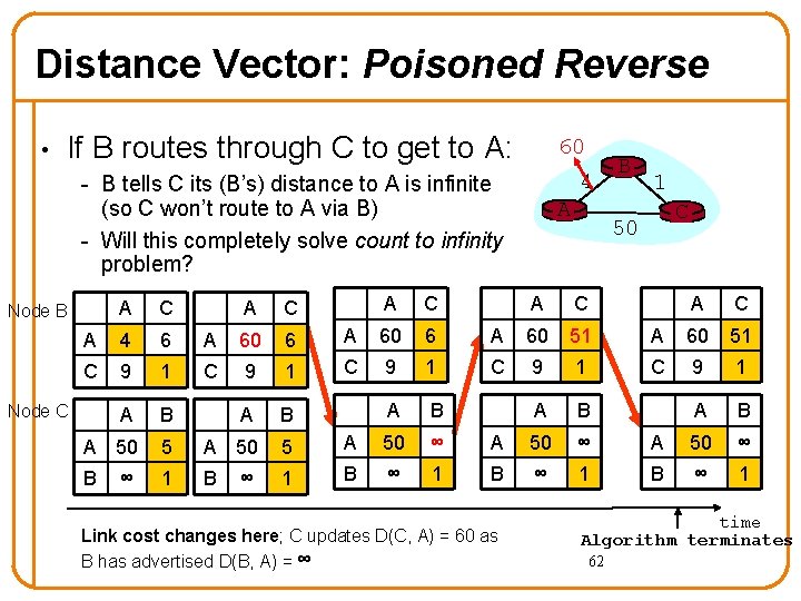
Distance Vector: Poisoned Reverse • If B routes through C to get to A: 60 4 - B tells C its (B’s) distance to A is infinite (so C won’t route to A via B) - Will this completely solve count to infinity problem? A C A 4 6 A 60 6 C 9 1 A B A 50 5 B 1 Node B Node C ∞ ∞ A C A 60 6 C 9 1 A B A 50 ∞ B ∞ 1 A 1 C 50 A C A 60 51 C 9 1 A B A 50 ∞ B ∞ 1 Link cost changes here; C updates D(C, A) = 60 as B has advertised D(B, A) = ∞ B A C A 60 51 C 9 1 A B A 50 ∞ B ∞ 1 time Algorithm terminates 62

Routing Information Protocol (RIP) • Simple distance-vector protocol – Nodes send distance vectors every 30 seconds – … or, when an update causes a change in routing • Link costs in RIP – All links have cost 1 – Valid distances of 1 through 15 – … with 16 representing infinity – Small “infinity” smaller “counting to infinity” problem • RIP is limited to fairly small networks – E. g. , campus 63

Question • Can we solve the count-to-infinity problem? • Do we need to solve the count-to-infinity problem? 64

Summary • Routing is a distributed algorithm – Different from forwarding – React to changes in the topology – Compute the shortest paths • Two main shortest-path algorithms – Dijkstra link-state routing (e. g. , OSPF, IS-IS) – Bellman-Ford distance-vector routing (e. g. , RIP) • Convergence process – Changing from one topology to another – Transient periods of inconsistency across routers • Next time: BGP – Reading: K&R 4. 6. 3 65