LMU talks 8 Kruskal Wallis nonparametric ANOVA ANOVA

LMU talks (8) Kruskal Wallis – nonparametric ANOVA

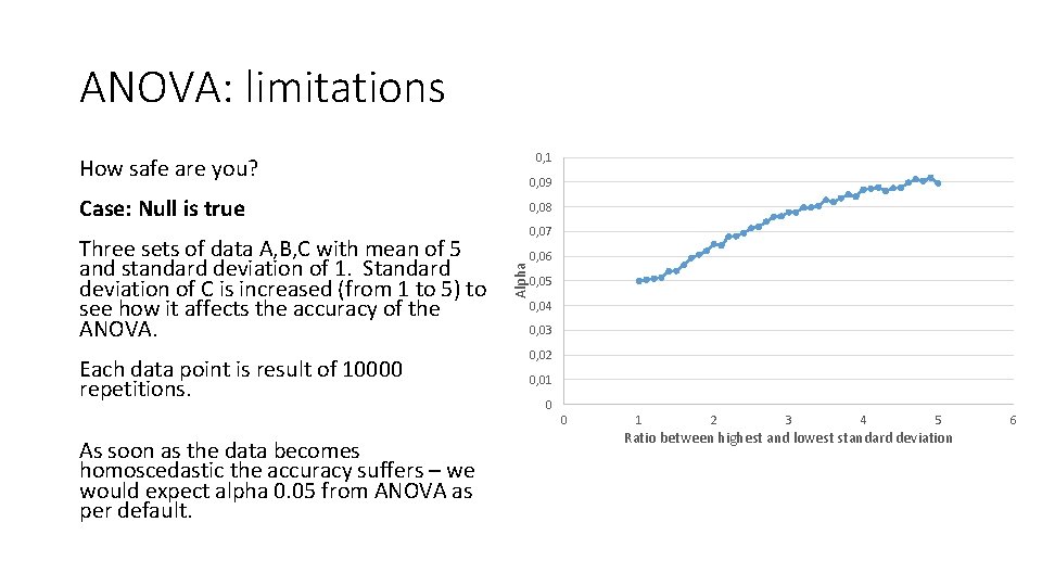
ANOVA: limitations 0, 1 How safe are you? 0, 09 Case: Null is true Each data point is result of 10000 repetitions. 0, 07 Alpha Three sets of data A, B, C with mean of 5 and standard deviation of 1. Standard deviation of C is increased (from 1 to 5) to see how it affects the accuracy of the ANOVA. 0, 08 0, 06 0, 05 0, 04 0, 03 0, 02 0, 01 0 0 As soon as the data becomes homoscedastic the accuracy suffers – we would expect alpha 0. 05 from ANOVA as per default. 1 2 3 4 5 Ratio between highest and lowest standard deviation 6

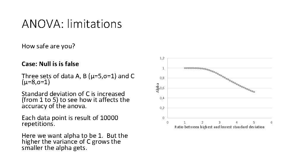
ANOVA: limitations How safe are you? 1, 2 Case: Null is is false Standard deviation of C is increased (from 1 to 5) to see how it affects the accuracy of the anova. Each data point is result of 10000 repetitions. Here we want alpha to be 1. But the higher the variance of C grows the smaller the alpha gets. 0, 8 Alpha Three sets of data A, B (μ=5, σ=1) and C (μ=8, σ=1) 1 0, 6 0, 4 0, 2 0 0 1 2 3 4 5 Ratio between highest and lowest standard deviation 6

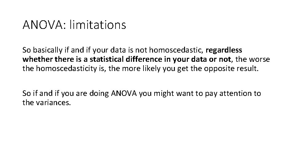
ANOVA: limitations So basically if and if your data is not homoscedastic, regardless whethere is a statistical difference in your data or not, the worse the homoscedasticity is, the more likely you get the opposite result. So if and if you are doing ANOVA you might want to pay attention to the variances.

ANOVA: limitations ANOVA (like most parametric models) does not really work when the data is homoscedastic. There’s some hand waving in the literature that if the smallest variance is no small than one third of the largest variance you are still safe. Which I only consider to be the case if null is true. But even this can be debated. But what if this isn’t the case? Kruskal-Wallis is your test.

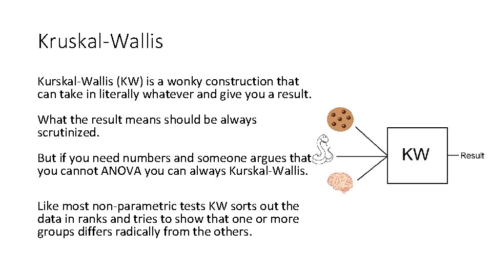
Kruskal-Wallis Kurskal-Wallis (KW) is a wonky construction that can take in literally whatever and give you a result. What the result means should be always scrutinized. But if you need numbers and someone argues that you cannot ANOVA you can always Kurskal-Wallis. Like most non-parametric tests KW sorts out the data in ranks and tries to show that one or more groups differs radically from the others.

Kurskal-Wallis Assumptions 1. Samples are random samples, or allocation to treatment group is random. 2. The samples are mutually independent. 3. The measurement scale is at least ordinal, and the variable is continuous. 4. If the test is used as a test of dominance, it has no distributional assumptions. If it is used to compare medians, the distributions must be similar apart from their locations. (Again, issues with variance) 5. The test is generally considered to be robust to ties. However, if ties are present they should not be concentrated together in one part of the distribution (they should have either a normal or uniform distribution) 6. N is at least 5 for each group. That being said that tables extend to groups that have N=1.

Stochastic Basically something randomly determined. From Greek, (stókhos) meaning a guess. Brownian motion is a stochastic process, i. e. the future state of the particle cannot be read from the past state.

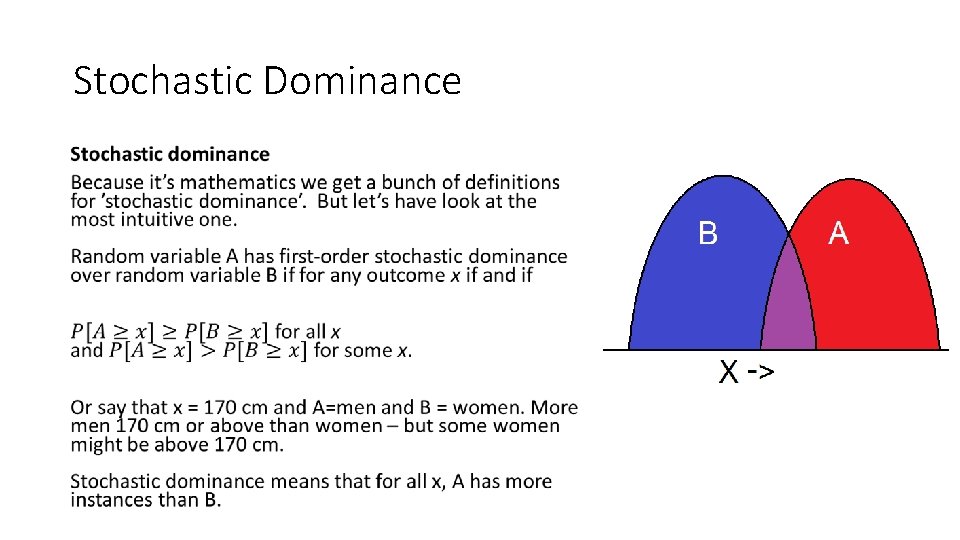
Stochastic Dominance •

Stochastic Dominance So yeah, stochastic dominance of a variable A over B just means that A is larger than B most of the time and B is never larger than A. You’ll note that Kurskal-Wallis makes no claims about mean. If the test result is significant if medians of the groups are ‘sufficiently’ different. As discussed before median might or might not be better measure than mean. But in biosciences people are stuck on means so, it’s good to keep in mind that Kurskal-Wallis is not about means.

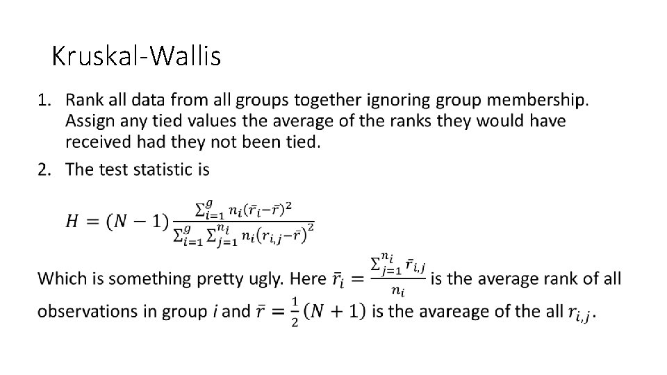
Kruskal-Wallis •

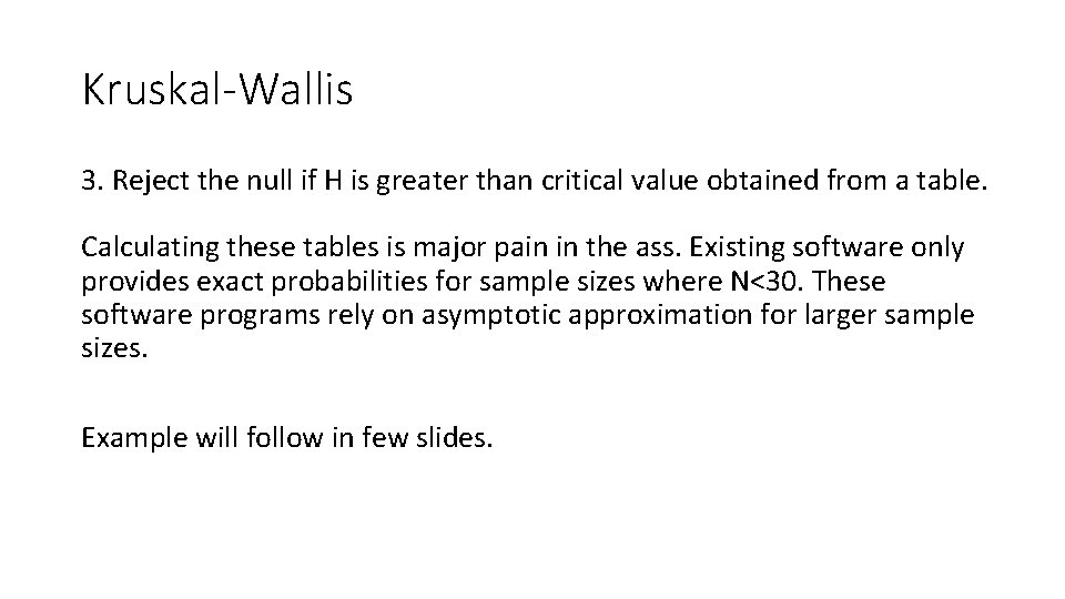
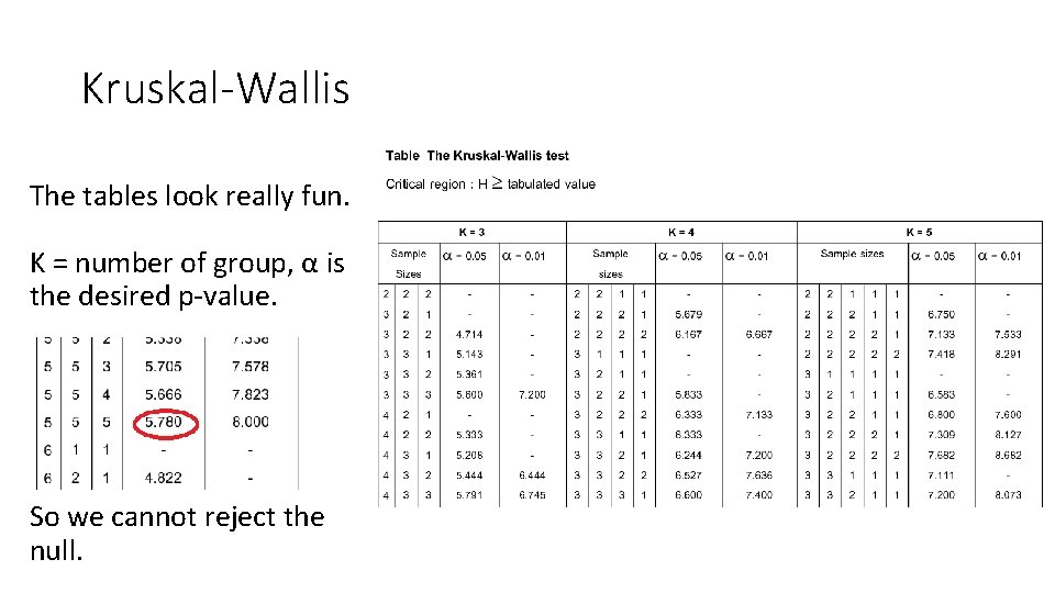
Kruskal-Wallis 3. Reject the null if H is greater than critical value obtained from a table. Calculating these tables is major pain in the ass. Existing software only provides exact probabilities for sample sizes where N<30. These software programs rely on asymptotic approximation for larger sample sizes. Example will follow in few slides.

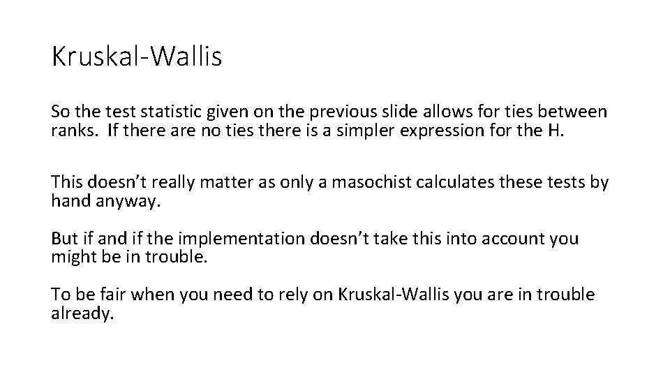
Kruskal-Wallis So the test statistic given on the previous slide allows for ties between ranks. If there are no ties there is a simpler expression for the H. This doesn’t really matter as only a masochist calculates these tests by hand anyway. But if and if the implementation doesn’t take this into account you might be in trouble. To be fair when you need to rely on Kruskal-Wallis you are in trouble already.

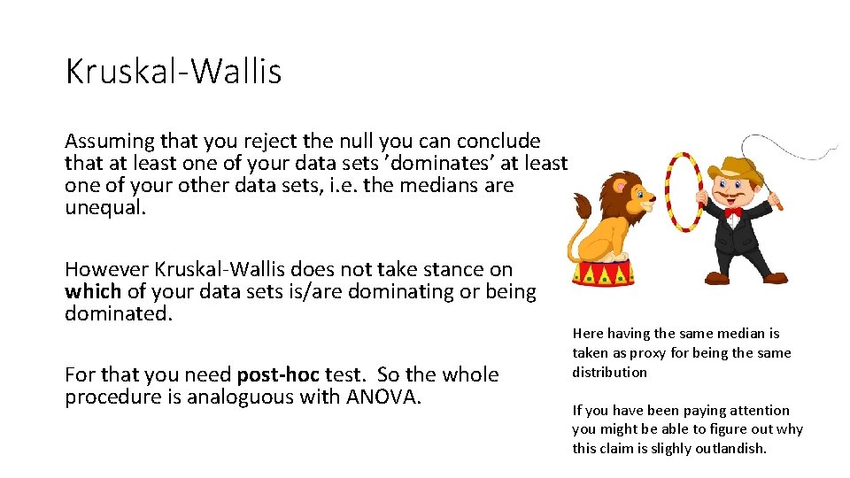
Kruskal-Wallis Assuming that you reject the null you can conclude that at least one of your data sets ’dominates’ at least one of your other data sets, i. e. the medians are unequal. However Kruskal-Wallis does not take stance on which of your data sets is/are dominating or being dominated. For that you need post-hoc test. So the whole procedure is analoguous with ANOVA. Here having the same median is taken as proxy for being the same distribution If you have been paying attention you might be able to figure out why this claim is slighly outlandish.

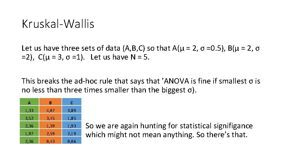
Kruskal-Wallis Let us have three sets of data (A, B, C) so that A(μ = 2, σ =0. 5), B(μ = 2, σ =2), C(μ = 3, σ =1). Let us have N = 5. This breaks the ad-hoc rule that says that ’ANOVA is fine if smallest σ is no less than three times smaller than the biggest σ). A B C 1, 33 4, 07 3, 89 3, 52 3, 45 1, 85 2, 36 1, 39 1, 93 1, 97 2, 59 2, 19 2, 36 0, 43 0, 06 So we are again hunting for statistical signifigance which might not mean anything. So there’s that.

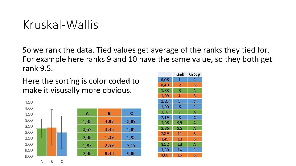
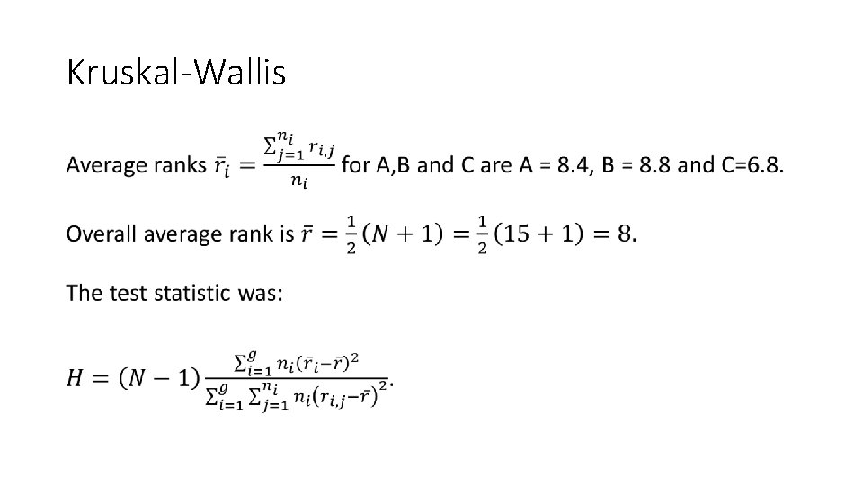
Kruskal-Wallis So we rank the data. Tied values get average of the ranks they tied for. For example here ranks 9 and 10 have the same value, so they both get rank 9. 5. Rank Group 0, 06 1 C Here the sorting is color coded to 0, 43 2 B 1, 33 3 A make it visusally more obvious. 4, 50 4, 00 3, 50 3, 00 2, 50 2, 00 1, 50 1, 00 0, 50 0, 00 A B C 1, 33 4, 07 3, 89 3, 52 3, 45 1, 85 2, 36 1, 39 1, 93 1, 97 2, 59 2, 19 2, 36 0, 43 0, 06 1, 39 1, 85 1, 93 1, 97 2, 19 2, 36 2, 59 3, 45 3, 52 3, 89 4, 07 4 5 6 7 8 9, 5 11 12 13 14 15 B C C A A B B A C B

Kruskal-Wallis •

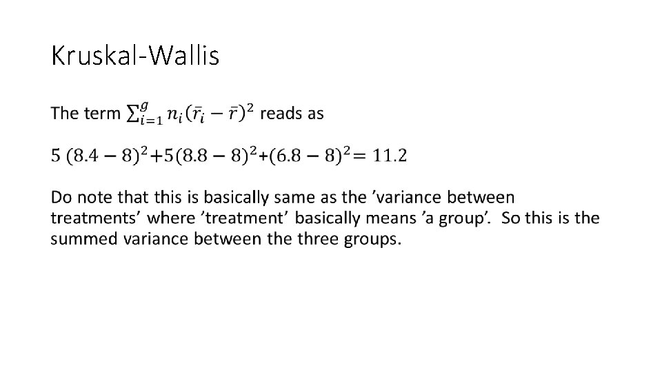
Kruskal-Wallis •

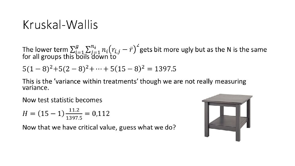
Kruskal-Wallis •

Kruskal-Wallis The tables look really fun. K = number of group, α is the desired p-value. So we cannot reject the null.

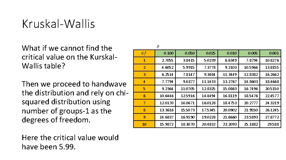
Kruskal-Wallis What if we cannot find the critical value on the Kurskal. Wallis table? Then we proceed to handwave the distribution and rely on chisquared distribution using number of groups-1 as the degrees of freedom. Here the critical value would have been 5. 99. p d. f 0. 100 0. 050 0. 025 0. 010 0. 005 0. 001 1 2. 7055 3. 8415 5. 0239 6. 6349 7. 8794 10. 8276 2 4. 6052 5. 9915 7. 3778 9. 2103 10. 5966 13. 8155 3 6. 2514 7. 8147 9. 3484 11. 3449 12. 8382 16. 2662 4 7. 7794 9. 4877 11. 1433 13. 2767 14. 8603 18. 4668 5 9. 2364 11. 0705 12. 8325 15. 0863 16. 7496 20. 5150 6 10. 6446 12. 5916 14. 4494 16. 8119 18. 5476 22. 4577 7 12. 0170 14. 0671 16. 0128 18. 4753 20. 2777 24. 3219 8 13. 3616 15. 5073 17. 5345 20. 0902 21. 9550 26. 1245 9 14. 6837 16. 9190 19. 0228 21. 6660 23. 5893 27. 8772 10 15. 9872 18. 3070 20. 4832 23. 2093 25. 1882 29. 588

Post-hoc Dunn’s test and Pairwise Mann-Whiteney

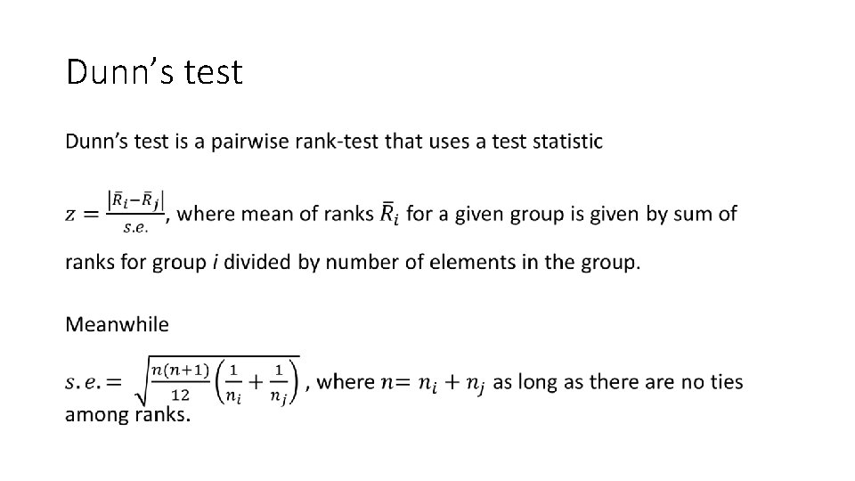
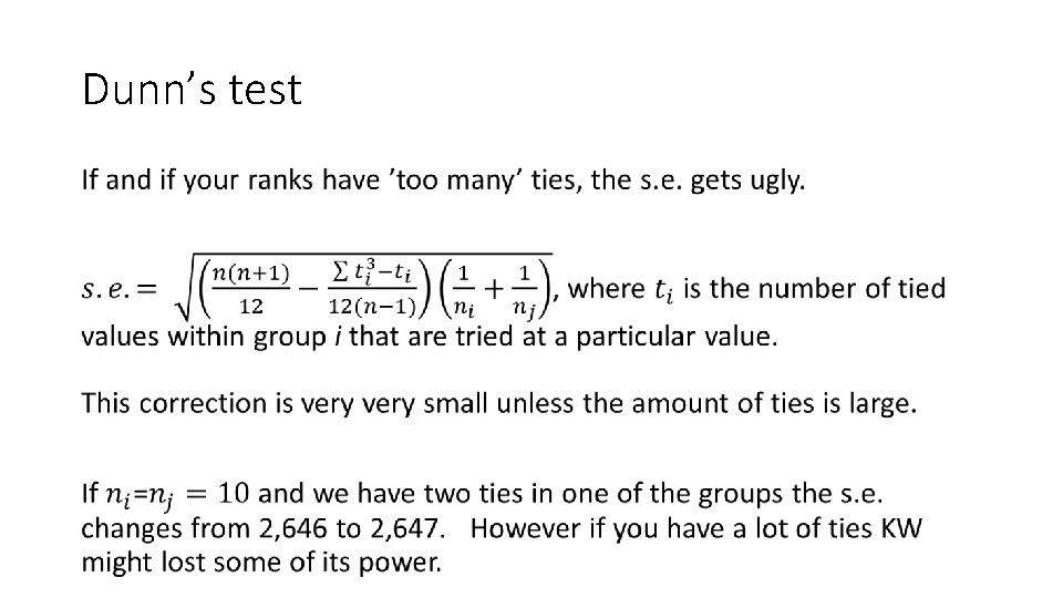
Dunn’s test

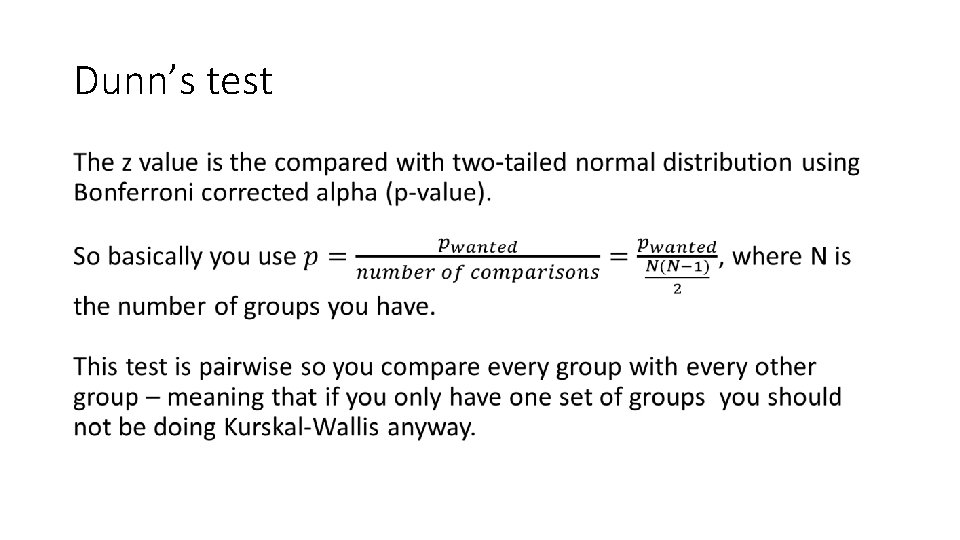
Dunn’s test •

Dunn’s test •

Dunn’s test •

Pairwise Mann-Whiteney

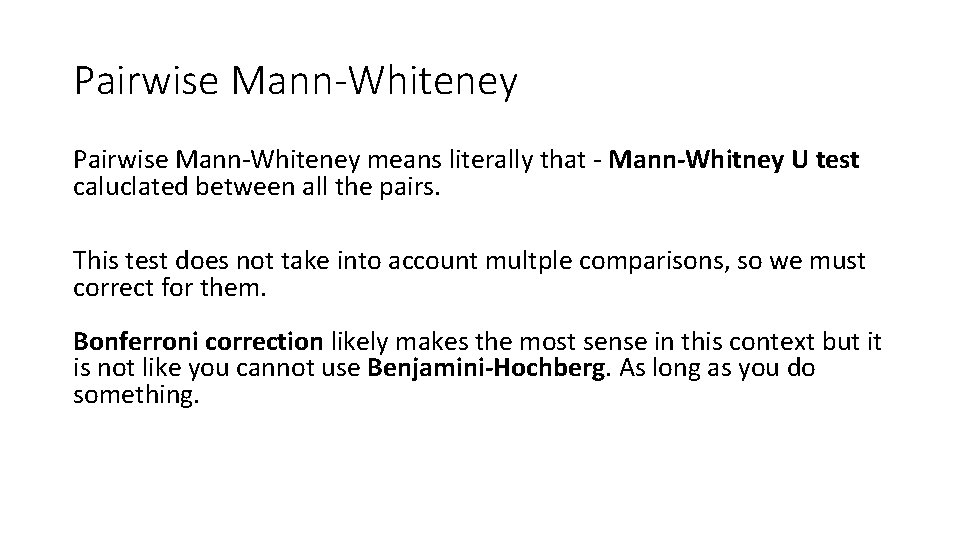
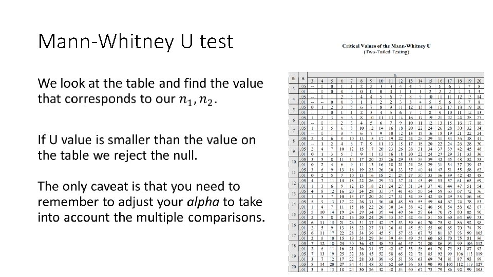
Pairwise Mann-Whiteney means literally that - Mann-Whitney U test caluclated between all the pairs. This test does not take into account multple comparisons, so we must correct for them. Bonferroni correction likely makes the most sense in this context but it is not like you cannot use Benjamini-Hochberg. As long as you do something.

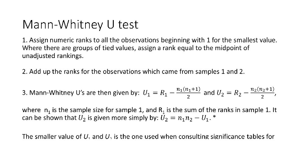
Mann-Whitney U test •

Mann-Whitney U test •

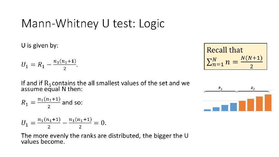
Mann-Whitney U test: Logic •

How about heteroscedastic data

Parametric ANOVA and heteroscedastic data To test Kurskal-Wallis against heteroscedasticity we need to create artificial data. Let us have uniformly distributed data with median m = 5 and σ = 1. Let us have samples A and B from this distribution. Then we make various samples of C with m = 5 but with σ that varies from 1. We shall call these C 1, C 2, C 3.

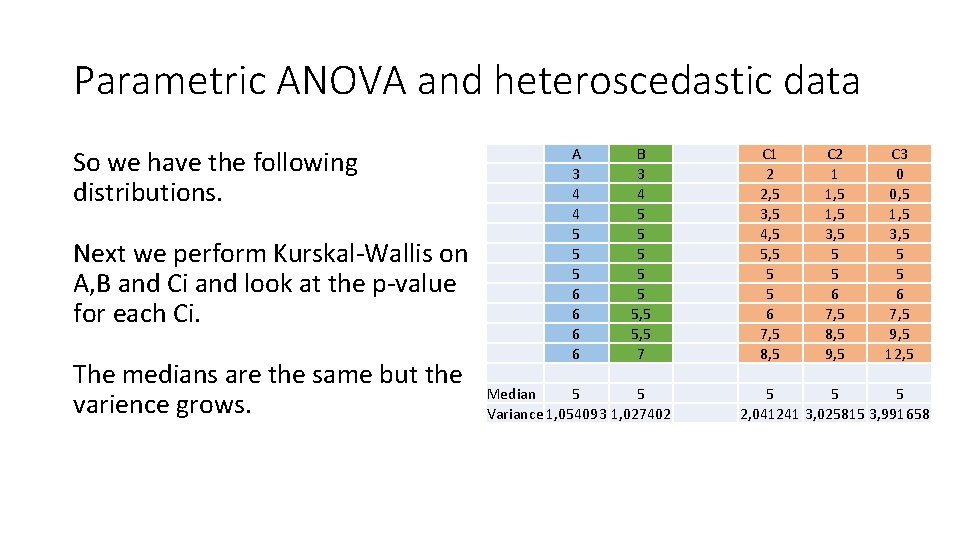
Parametric ANOVA and heteroscedastic data So we have the following distributions. Next we perform Kurskal-Wallis on A, B and Ci and look at the p-value for each Ci. The medians are the same but the varience grows. A 3 4 4 5 5 5 6 6 B 3 4 5 5 5, 5 7 Median 5 5 Variance 1, 054093 1, 027402 C 1 2 2, 5 3, 5 4, 5 5 5 6 7, 5 8, 5 C 2 1 1, 5 3, 5 5 5 6 7, 5 8, 5 9, 5 C 3 0 0, 5 1, 5 3, 5 5 5 6 7, 5 9, 5 12, 5 5 2, 041241 3, 025815 3, 991658

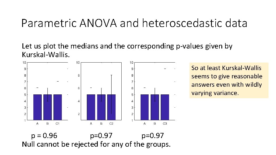
Parametric ANOVA and heteroscedastic data Let us plot the medians and the corresponding p-values given by Kurskal-Wallis. So at least Kurskal-Wallis seems to give reasonable answers even with wildly varying variance. p = 0. 96 p=0. 97 Null cannot be rejected for any of the groups.

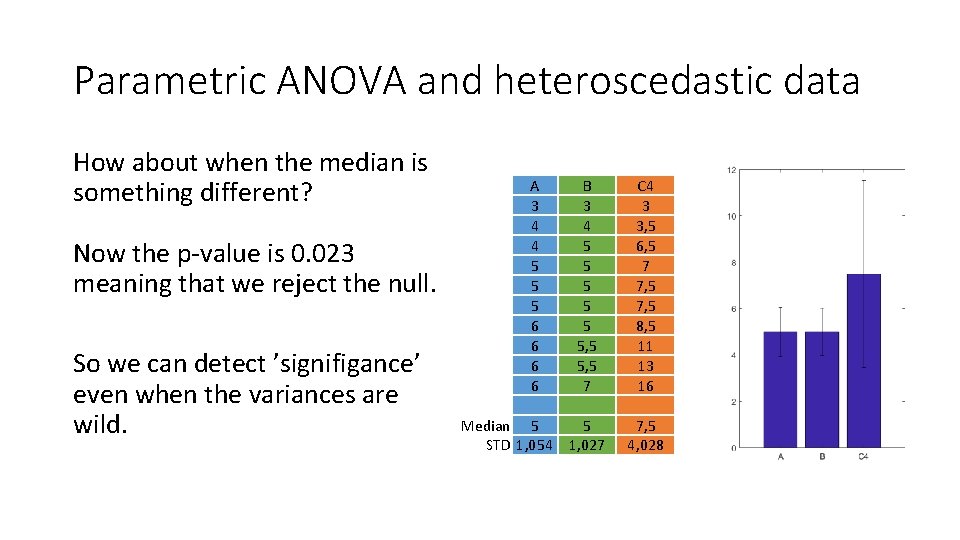
Parametric ANOVA and heteroscedastic data How about when the median is something different? Now the p-value is 0. 023 meaning that we reject the null. So we can detect ’signifigance’ even when the variances are wild. A 3 4 4 5 5 5 6 6 B 3 4 5 5 5, 5 7 Median 5 5 STD 1, 054 1, 027 C 4 3 3, 5 6, 5 7 7, 5 8, 5 11 13 16 7, 5 4, 028

Philosophy

Philosophy Kurskal-Wallis offers an insight why some mathematicians consider statistics branch of philosophy rather than mathematics. The math itself can be justified, it is the axioms that are disconnected from reality. Consider the following. If we measure something in the nature and the medians of the two sets of measurements are the same, but the standard deviation is not – are the two things really different or the same? How can we know? When are the standard deviations different enough to warrant us calling the samples ’different’? What in life is truly objective and not subjective? Do we have a free will? What is the difference between good and evil?

Next time Bootstrap!