Lecture 10 Ftests in MLR continued Coefficients of

Lecture 10 F-tests in MLR (continued) Coefficients of Determination BMTRY 701 Biostatistical Methods II

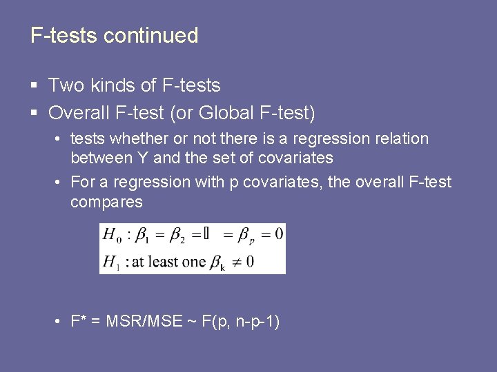
F-tests continued § Two kinds of F-tests § Overall F-test (or Global F-test) • tests whether or not there is a regression relation between Y and the set of covariates • For a regression with p covariates, the overall F-test compares • F* = MSR/MSE ~ F(p, n-p-1)

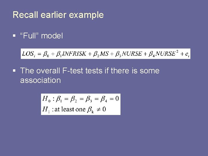
Recall earlier example § “Full” model § The overall F-tests if there is some association

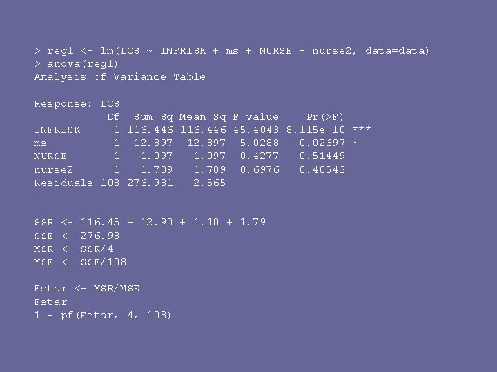
> reg 1 <- lm(LOS ~ INFRISK + ms + NURSE + nurse 2, data=data) > anova(reg 1) Analysis of Variance Table Response: LOS Df Sum Sq Mean Sq F value Pr(>F) INFRISK 1 116. 446 45. 4043 8. 115 e-10 *** ms 1 12. 897 5. 0288 0. 02697 * NURSE 1 1. 097 0. 4277 0. 51449 nurse 2 1 1. 789 0. 6976 0. 40543 Residuals 108 276. 981 2. 565 --SSR SSE MSR MSE <<<<- 116. 45 + 12. 90 + 1. 10 + 1. 79 276. 98 SSR/4 SSE/108 Fstar <- MSR/MSE Fstar 1 - pf(Fstar, 4, 108)

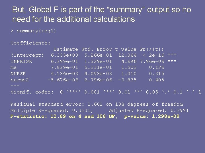
But, Global F is part of the “summary” output so no need for the additional calculations > summary(reg 1) Coefficients: Estimate Std. Error t value Pr(>|t|) (Intercept) 6. 355 e+00 5. 266 e-01 12. 068 < 2 e-16 *** INFRISK 6. 289 e-01 1. 339 e-01 4. 696 7. 86 e-06 *** ms 7. 829 e-01 5. 211 e-01 1. 502 0. 136 NURSE 4. 136 e-03 4. 093 e-03 1. 010 0. 315 nurse 2 -5. 676 e-06 6. 796 e-06 -0. 835 0. 405 --Signif. codes: 0 ‘***’ 0. 001 ‘**’ 0. 01 ‘*’ 0. 05 ‘. ’ 0. 1 ‘ ’ 1 Residual standard error: 1. 601 on 108 degrees of freedom Multiple R-squared: 0. 3231, Adjusted R-squared: 0. 2981 F-statistic: 12. 89 on 4 and 108 DF, p-value: 1. 298 e-08

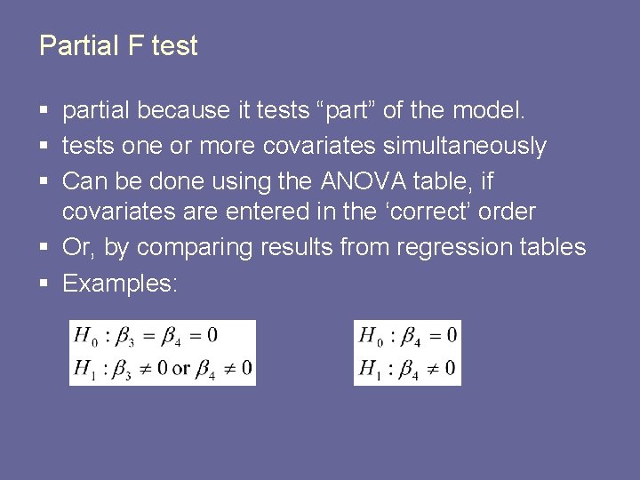
Partial F test § partial because it tests “part” of the model. § tests one or more covariates simultaneously § Can be done using the ANOVA table, if covariates are entered in the ‘correct’ order § Or, by comparing results from regression tables § Examples:

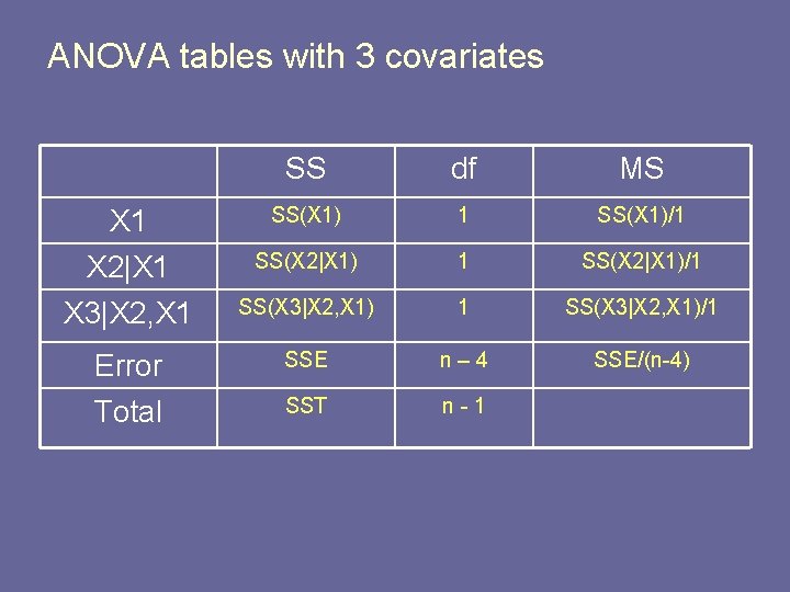
ANOVA tables with 3 covariates SS df MS X 1 X 2|X 1 SS(X 1)/1 SS(X 2|X 1)/1 X 3|X 2, X 1 SS(X 3|X 2, X 1)/1 Error Total SSE n– 4 SSE/(n-4) SST n-1

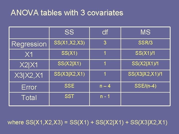
ANOVA tables with 3 covariates SS df MS Regression X 1 SS(X 1, X 2, X 3) 3 SSR/3 SS(X 1) 1 SS(X 1)/1 X 2|X 1 SS(X 2|X 1)/1 X 3|X 2, X 1 SS(X 3|X 2, X 1)/1 Error Total SSE n– 4 SSE/(n-4) SST n-1 where SS(X 1, X 2, X 3) = SS(X 1) + SS(X 2|X 1) + SS(X 3|X 2, X 1)

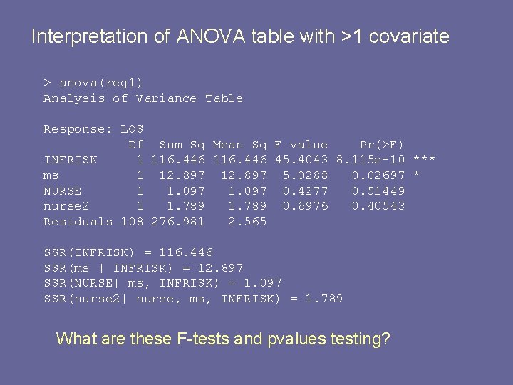
Interpretation of ANOVA table with >1 covariate > anova(reg 1) Analysis of Variance Table Response: LOS Df Sum Sq Mean Sq F value Pr(>F) INFRISK 1 116. 446 45. 4043 8. 115 e-10 *** ms 1 12. 897 5. 0288 0. 02697 * NURSE 1 1. 097 0. 4277 0. 51449 nurse 2 1 1. 789 0. 6976 0. 40543 Residuals 108 276. 981 2. 565 SSR(INFRISK) = 116. 446 SSR(ms | INFRISK) = 12. 897 SSR(NURSE| ms, INFRISK) = 1. 097 SSR(nurse 2| nurse, ms, INFRISK) = 1. 789 What are these F-tests and pvalues testing?

F-tests and p-values in ANOVA table § They are tests for a covariate, conditional on what is above it in the table. § Example: • F statistic for INFRISK tests • is it adjusted for other covariates? § no § it tests INFRISK in the presence of no other covariates § p < 0. 0001

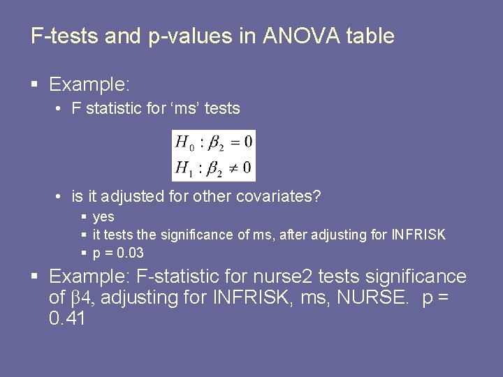
F-tests and p-values in ANOVA table § Example: • F statistic for ‘ms’ tests • is it adjusted for other covariates? § yes § it tests the significance of ms, after adjusting for INFRISK § p = 0. 03 § Example: F-statistic for nurse 2 tests significance of β 4, adjusting for INFRISK, ms, NURSE. p = 0. 41

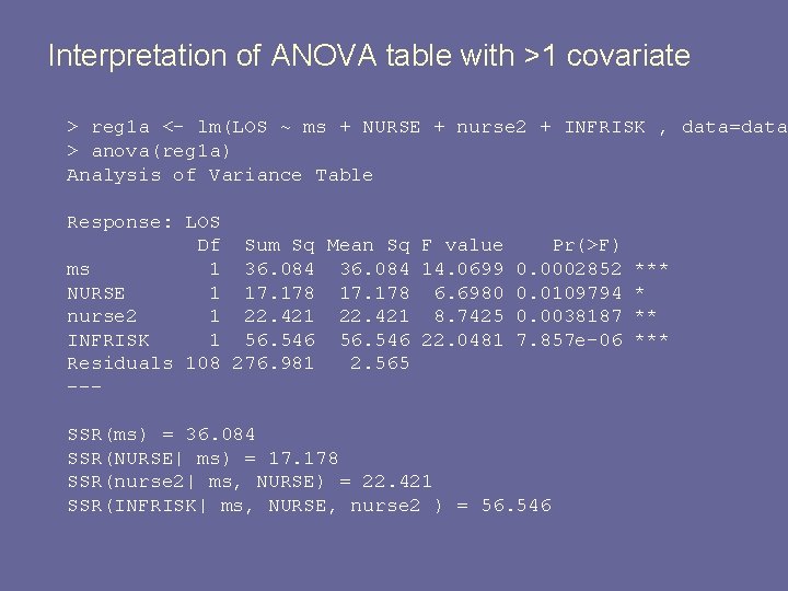
Interpretation of ANOVA table with >1 covariate > reg 1 a <- lm(LOS ~ ms + NURSE + nurse 2 + INFRISK , data=data > anova(reg 1 a) Analysis of Variance Table Response: LOS Df Sum Sq Mean Sq F value Pr(>F) ms 1 36. 084 14. 0699 0. 0002852 *** NURSE 1 17. 178 6. 6980 0. 0109794 * nurse 2 1 22. 421 8. 7425 0. 0038187 ** INFRISK 1 56. 546 22. 0481 7. 857 e-06 *** Residuals 108 276. 981 2. 565 --SSR(ms) = 36. 084 SSR(NURSE| ms) = 17. 178 SSR(nurse 2| ms, NURSE) = 22. 421 SSR(INFRISK| ms, NURSE, nurse 2 ) = 56. 546

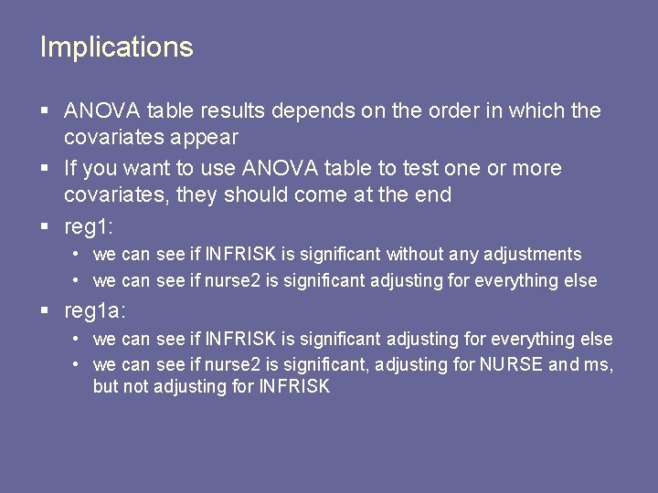
Implications § ANOVA table results depends on the order in which the covariates appear § If you want to use ANOVA table to test one or more covariates, they should come at the end § reg 1: • we can see if INFRISK is significant without any adjustments • we can see if nurse 2 is significant adjusting for everything else § reg 1 a: • we can see if INFRISK is significant adjusting for everything else • we can see if nurse 2 is significant, adjusting for NURSE and ms, but not adjusting for INFRISK

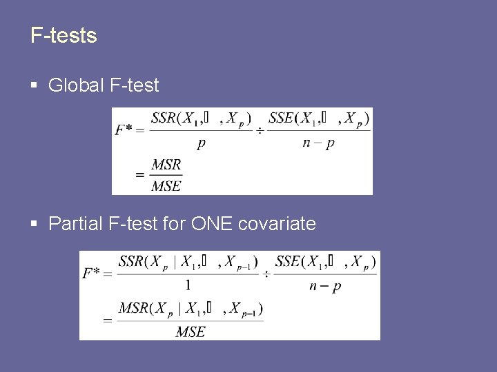
F-tests § Global F-test § Partial F-test for ONE covariate

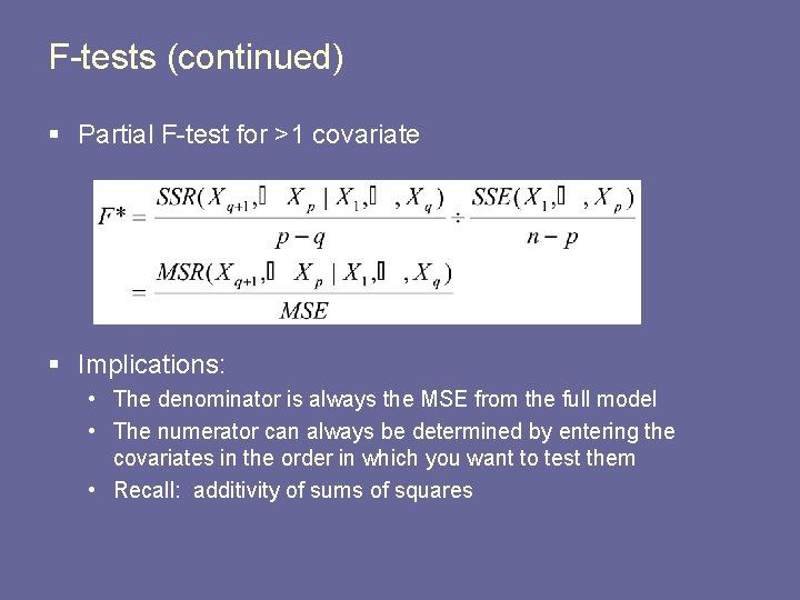
F-tests (continued) § Partial F-test for >1 covariate § Implications: • The denominator is always the MSE from the full model • The numerator can always be determined by entering the covariates in the order in which you want to test them • Recall: additivity of sums of squares

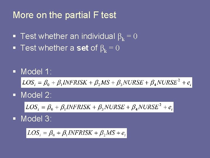
More on the partial F test § Test whether an individual βk = 0 § Test whether a set of βk = 0 § Model 1: § Model 2: § Model 3:

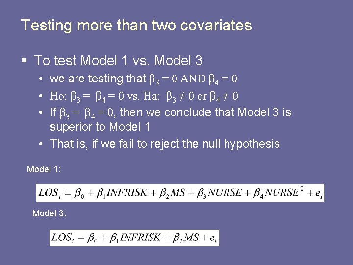
Testing more than two covariates § To test Model 1 vs. Model 3 • we are testing that β 3 = 0 AND β 4 = 0 • Ho: β 3 = β 4 = 0 vs. Ha: β 3 ≠ 0 or β 4 ≠ 0 • If β 3 = β 4 = 0, then we conclude that Model 3 is superior to Model 1 • That is, if we fail to reject the null hypothesis Model 1: Model 3:

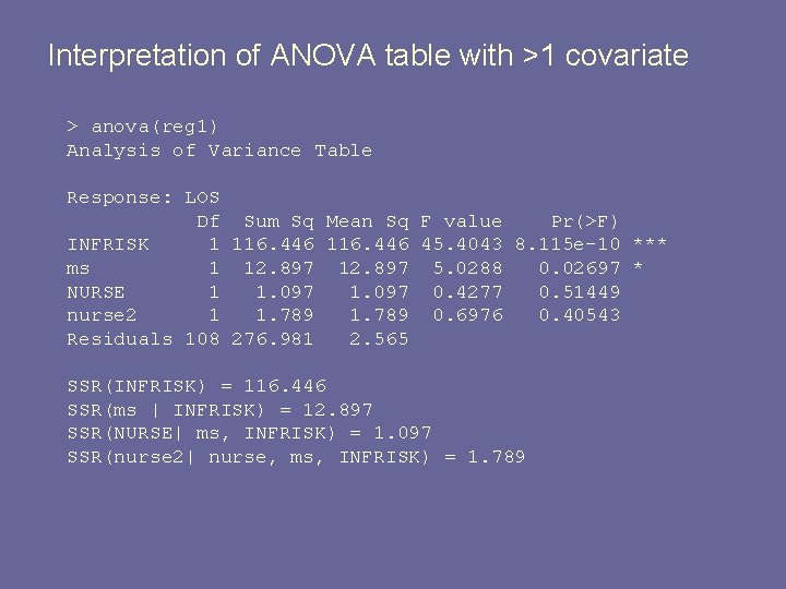
Interpretation of ANOVA table with >1 covariate > anova(reg 1) Analysis of Variance Table Response: LOS Df Sum Sq Mean Sq F value Pr(>F) INFRISK 1 116. 446 45. 4043 8. 115 e-10 *** ms 1 12. 897 5. 0288 0. 02697 * NURSE 1 1. 097 0. 4277 0. 51449 nurse 2 1 1. 789 0. 6976 0. 40543 Residuals 108 276. 981 2. 565 SSR(INFRISK) = 116. 446 SSR(ms | INFRISK) = 12. 897 SSR(NURSE| ms, INFRISK) = 1. 097 SSR(nurse 2| nurse, ms, INFRISK) = 1. 789

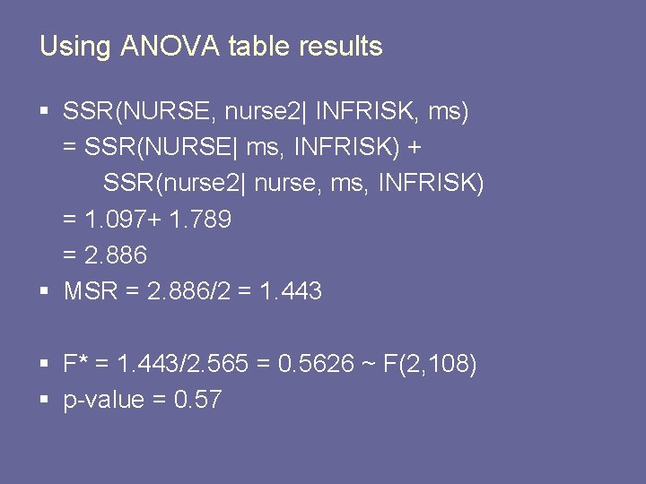
Using ANOVA table results § SSR(NURSE, nurse 2| INFRISK, ms) = SSR(NURSE| ms, INFRISK) + SSR(nurse 2| nurse, ms, INFRISK) = 1. 097+ 1. 789 = 2. 886 § MSR = 2. 886/2 = 1. 443 § F* = 1. 443/2. 565 = 0. 5626 ~ F(2, 108) § p-value = 0. 57

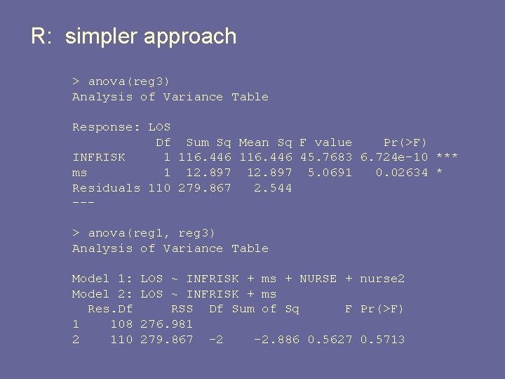
R: simpler approach > anova(reg 3) Analysis of Variance Table Response: LOS Df Sum Sq Mean Sq F value Pr(>F) INFRISK 1 116. 446 45. 7683 6. 724 e-10 *** ms 1 12. 897 5. 0691 0. 02634 * Residuals 110 279. 867 2. 544 --> anova(reg 1, reg 3) Analysis of Variance Table Model 1: Model 2: Res. Df 1 108 2 110 LOS ~ INFRISK + ms + NURSE + nurse 2 LOS ~ INFRISK + ms RSS Df Sum of Sq F Pr(>F) 276. 981 279. 867 -2 -2. 886 0. 5627 0. 5713

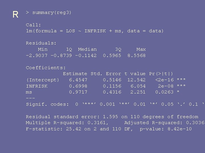
R > summary(reg 3) Call: lm(formula = LOS ~ INFRISK + ms, data = data) Residuals: Min 1 Q Median -2. 9037 -0. 8739 -0. 1142 3 Q 0. 5965 Max 8. 5568 Coefficients: Estimate Std. Error t value Pr(>|t|) (Intercept) 6. 4547 0. 5146 12. 542 <2 e-16 *** INFRISK 0. 6998 0. 1156 6. 054 2 e-08 *** ms 0. 9717 0. 4316 2. 251 0. 0263 * --Signif. codes: 0 ‘***’ 0. 001 ‘**’ 0. 01 ‘*’ 0. 05 ‘. ’ 0. 1 ‘ Residual standard error: 1. 595 on 110 degrees of freedom Multiple R-squared: 0. 3161, Adjusted R-squared: 0. 3036 F-statistic: 25. 42 on 2 and 110 DF, p-value: 8. 42 e-10

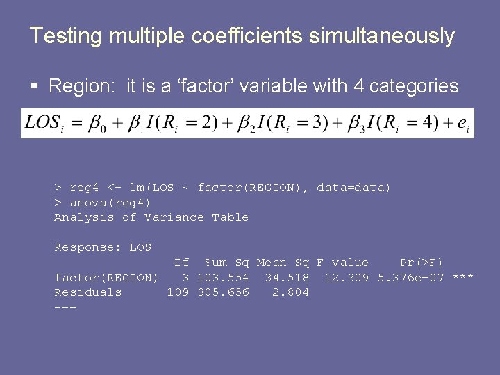
Testing multiple coefficients simultaneously § Region: it is a ‘factor’ variable with 4 categories > reg 4 <- lm(LOS ~ factor(REGION), data=data) > anova(reg 4) Analysis of Variance Table Response: LOS Df Sum Sq Mean Sq F value Pr(>F) factor(REGION) 3 103. 554 34. 518 12. 309 5. 376 e-07 *** Residuals 109 305. 656 2. 804 ---

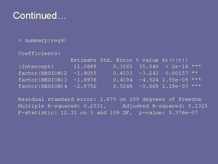
Continued… > summary(reg 4) Coefficients: Estimate Std. Error t value Pr(>|t|) (Intercept) 11. 0889 0. 3165 35. 040 < 2 e-16 *** factor(REGION)2 -1. 4055 0. 4333 -3. 243 0. 00157 ** factor(REGION)3 -1. 8976 0. 4194 -4. 524 1. 55 e-05 *** factor(REGION)4 -2. 9752 0. 5248 -5. 669 1. 19 e-07 *** Residual standard error: 1. 675 on 109 degrees of freedom Multiple R-squared: 0. 2531, Adjusted R-squared: 0. 2325 F-statistic: 12. 31 on 3 and 109 DF, p-value: 5. 376 e-07

Recall previous example § Interaction between REGION and MEDSCHL

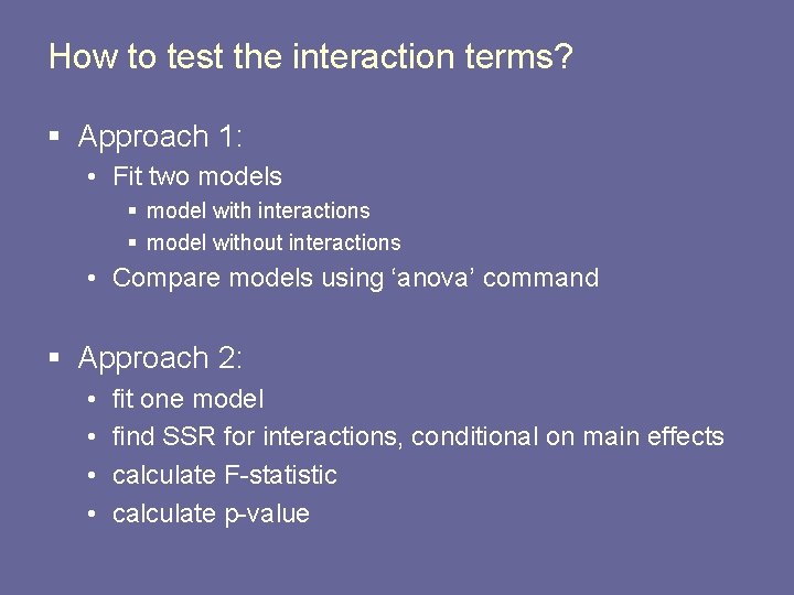
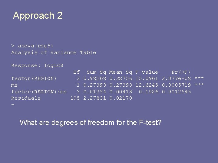
How to test the interaction terms? § Approach 1: • Fit two models § model with interactions § model without interactions • Compare models using ‘anova’ command § Approach 2: • • fit one model find SSR for interactions, conditional on main effects calculate F-statistic calculate p-value

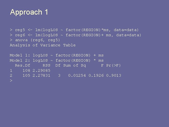
Approach 1 > reg 5 <- lm(log. LOS ~ factor(REGION)*ms, data=data) > reg 6 <- lm(log. LOS ~ factor(REGION)+ ms, data=data) > anova (reg 6, reg 5) Analysis of Variance Table Model 1: Model 2: Res. Df 1 108 2 105 > log. LOS ~ factor(REGION) + ms log. LOS ~ factor(REGION) * ms RSS Df Sum of Sq F Pr(>F) 2. 29085 2. 27831 3 0. 01254 0. 1926 0. 9013

Approach 2 > anova(reg 5) Analysis of Variance Table Response: log. LOS Df factor(REGION) 3 ms 1 factor(REGION): ms 3 Residuals 105 - Sum Sq 0. 98268 0. 27393 0. 01254 2. 27831 Mean Sq F value Pr(>F) 0. 32756 15. 0961 3. 077 e-08 *** 0. 27393 12. 6245 0. 0005719 *** 0. 00418 0. 1926 0. 9012545 0. 02170 What are degrees of freedom for the F-test?

Concluding remarks r. e. F-test § Global F-test: not very common, except for very small models § Partial F-test for individual covariate: not very common because it is the same as the t-test § Partial F-test for set of covariates: • quite common • easiest to find ANOVA table for nested models • can use ANOVA table from full model to determine Fstatistic

Coefficient of Determination § Also called R 2 § Measures the variability in Y explained by the covariates. § Two questions (and think ‘sums of squares’ in ANOVA): • How do we measure the variance in Y? • How do we measure the variance explained by the X’s?

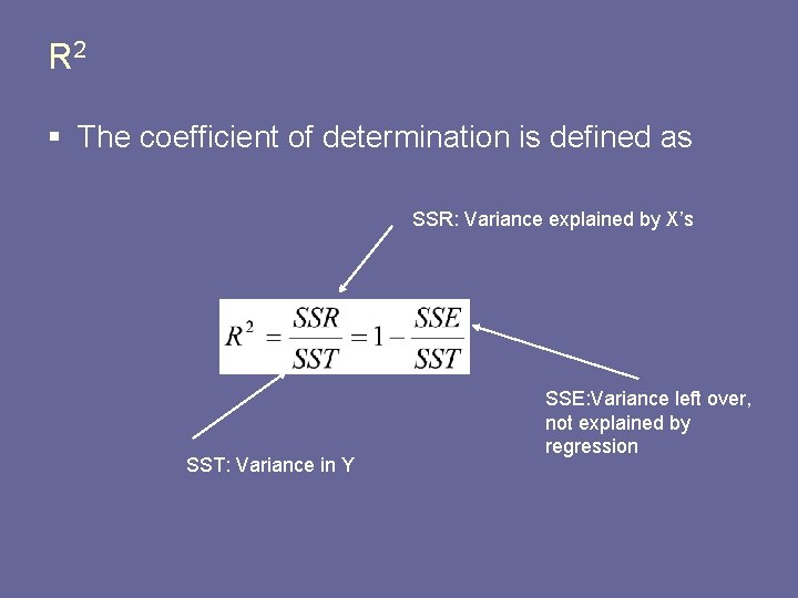
R 2 § The coefficient of determination is defined as SSR: Variance explained by X’s SST: Variance in Y SSE: Variance left over, not explained by regression

Use of R 2 § § Similar to correlation But, not specific to just one X and Y Partitioning of explained versus unexplained For certain models, it can be used to determine if addition of a covariate helps ‘predict’

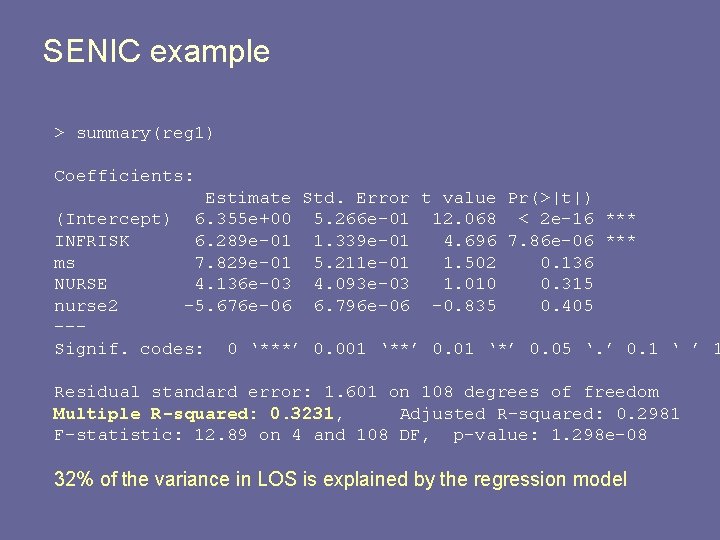
SENIC example > summary(reg 1) Coefficients: Estimate Std. Error t value Pr(>|t|) (Intercept) 6. 355 e+00 5. 266 e-01 12. 068 < 2 e-16 *** INFRISK 6. 289 e-01 1. 339 e-01 4. 696 7. 86 e-06 *** ms 7. 829 e-01 5. 211 e-01 1. 502 0. 136 NURSE 4. 136 e-03 4. 093 e-03 1. 010 0. 315 nurse 2 -5. 676 e-06 6. 796 e-06 -0. 835 0. 405 --Signif. codes: 0 ‘***’ 0. 001 ‘**’ 0. 01 ‘*’ 0. 05 ‘. ’ 0. 1 ‘ ’ 1 Residual standard error: 1. 601 on 108 degrees of freedom Multiple R-squared: 0. 3231, Adjusted R-squared: 0. 2981 F-statistic: 12. 89 on 4 and 108 DF, p-value: 1. 298 e-08 32% of the variance in LOS is explained by the regression model

Misunderstandings r. e. R 2 § A high R 2 indicates that a useful prediction can be made • there still may be considerable uncertainty, due to small N. • recall that predictions depend on how close “X” is to the mean § A high R 2 indicates that the regression model is a ‘good fit’ • high R 2 says nothing about adhering to model assumptions • standard diagnostics should still be used, even if R 2 is high § R 2 near 0 indicates X and Y are not related. • for similar reasons as above, need to look at modeling • X and Y may be related, but not linearly

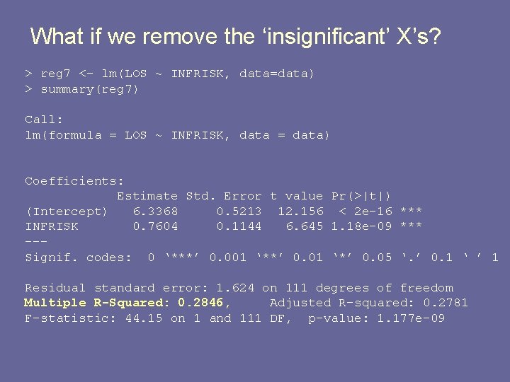
What if we remove the ‘insignificant’ X’s? > reg 7 <- lm(LOS ~ INFRISK, data=data) > summary(reg 7) Call: lm(formula = LOS ~ INFRISK, data = data) Coefficients: Estimate Std. Error t value Pr(>|t|) (Intercept) 6. 3368 0. 5213 12. 156 < 2 e-16 *** INFRISK 0. 7604 0. 1144 6. 645 1. 18 e-09 *** --Signif. codes: 0 ‘***’ 0. 001 ‘**’ 0. 01 ‘*’ 0. 05 ‘. ’ 0. 1 ‘ ’ 1 Residual standard error: 1. 624 on 111 degrees of freedom Multiple R-Squared: 0. 2846, Adjusted R-squared: 0. 2781 F-statistic: 44. 15 on 1 and 111 DF, p-value: 1. 177 e-09

R 2 decreased? § The addition of a covariate will ALWAYS increase the R 2 value. § Why? • there is always at least a little bit explained by the new X • the only possible way to have no increase in R 2 would be if the addition of the new covariate had estimated β = 0 • It is ‘almost never’ true that the slope estimate is exactly. § Extreme case: • perfect linear association between two covariates (e. g. , age in years and age in months)

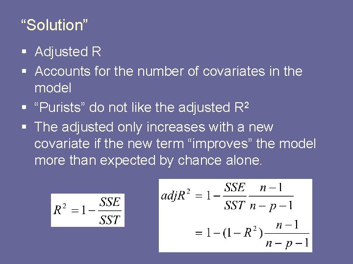
“Solution” § Adjusted R § Accounts for the number of covariates in the model § “Purists” do not like the adjusted R 2 § The adjusted only increases with a new covariate if the new term “improves” the model more than expected by chance alone.

Coefficients of Partial Determination § Measures the marginal contribution of one X variable when all others are already in the model § Intuitively, how much variation in Y are we explaining, after accounting for what is already in the model? § Construction in Two Covariate case:

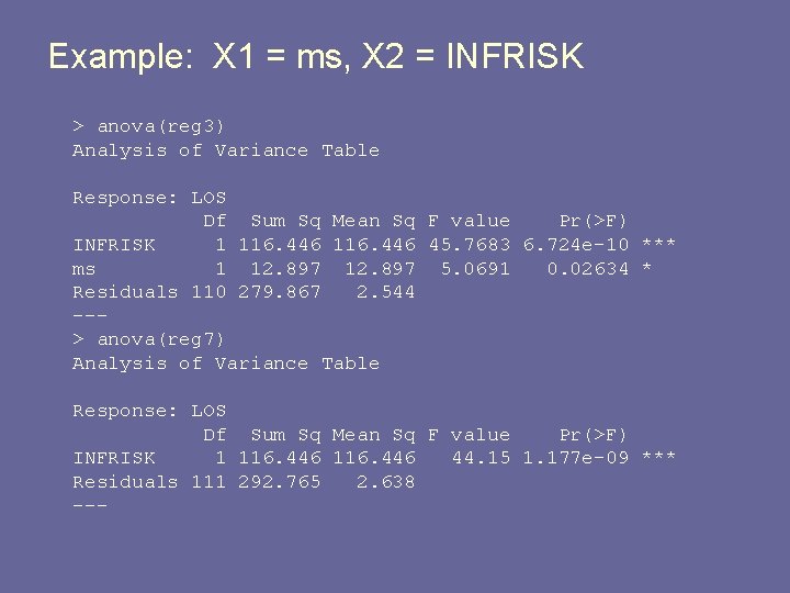
Example: X 1 = ms, X 2 = INFRISK > anova(reg 3) Analysis of Variance Table Response: LOS Df Sum Sq Mean Sq F value Pr(>F) INFRISK 1 116. 446 45. 7683 6. 724 e-10 *** ms 1 12. 897 5. 0691 0. 02634 * Residuals 110 279. 867 2. 544 --> anova(reg 7) Analysis of Variance Table Response: LOS Df Sum Sq Mean Sq F value Pr(>F) INFRISK 1 116. 446 44. 15 1. 177 e-09 *** Residuals 111 292. 765 2. 638 ---

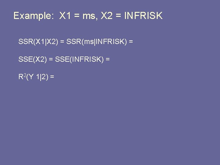
Example: X 1 = ms, X 2 = INFRISK SSR(X 1|X 2) = SSR(ms|INFRISK) = SSE(X 2) = SSE(INFRISK) = R 2(Y 1|2) =

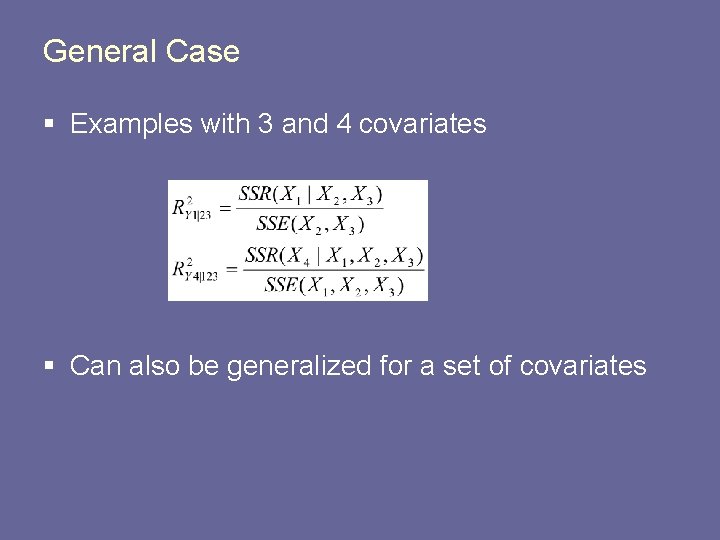
General Case § Examples with 3 and 4 covariates § Can also be generalized for a set of covariates