Lecture 1 MGMT 650 Management Science and Decision

Lecture 1 MGMT 650 Management Science and Decision Analysis

Agenda Operations Management n Chapter 1 • Management Science & relation to OM • Quantitative Analysis and Decision Making • Cost, Revenue, and Profit Models • Management Science Techniques • Introduction to Linear Programming n 2

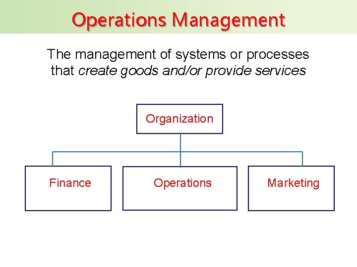
Operations Management The management of systems or processes that create goods and/or provide services Organization Finance Operations Marketing

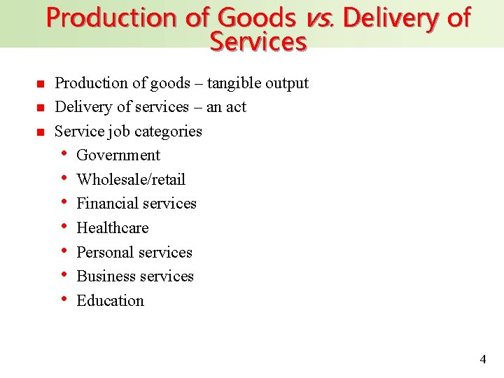
Production of Goods vs. Delivery of Services n n n Production of goods – tangible output Delivery of services – an act Service job categories • Government • Wholesale/retail • Financial services • Healthcare • Personal services • Business services • Education 4

Scope of Operations Management n n Operations Management includes: • Forecasting • Capacity planning • Scheduling • Managing inventories • Assuring quality • Deciding where to locate facilities • And more. . . The operations function • Consists of all activities directly related to producing goods or providing services 5

Management Science The body of knowledge involving quantitative approaches to decision making is referred to as • Management Science • Operations research • Decision science n It had its early roots in World War II and is flourishing in business and industry with the aid of computers n 6

Problem Solving and Decision Making n Steps of Problem Solving (First 5 steps are the process of decision making) • Define the problem. • Identify the set of alternative solutions. • Determine the criteria for evaluating alternatives. • Evaluate the alternatives. • Choose an alternative (make a decision). ---------------------------------- • Implement the chosen alternative. • Evaluate the results. 7

Quantitative Analysis and Decision Making n Potential Reasons for a Quantitative Analysis Approach to Decision Making • The problem is complex • The problem is very important • The problem is new • The problem is repetitive 8

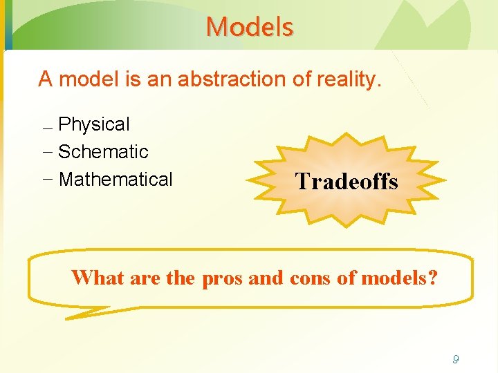
Models A model is an abstraction of reality. – Physical – Schematic – Mathematical Tradeoffs What are the pros and cons of models? 9

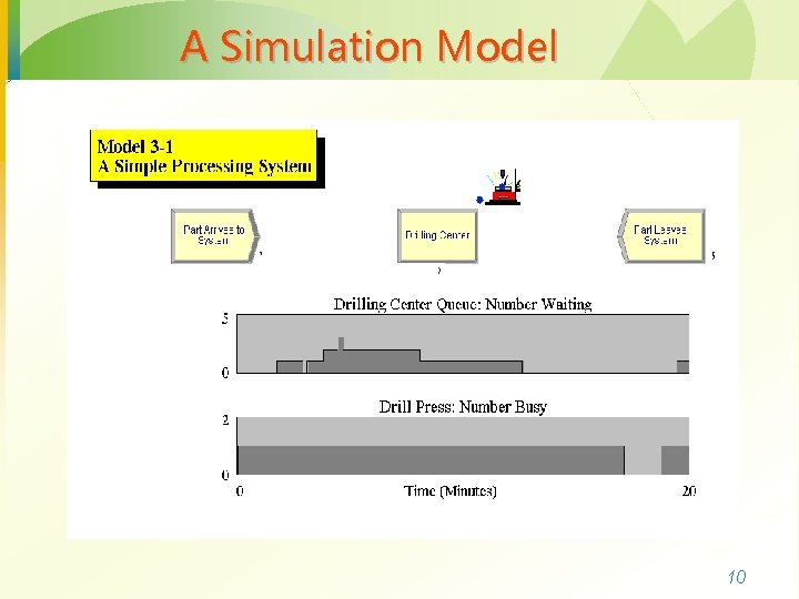
A Simulation Model 10

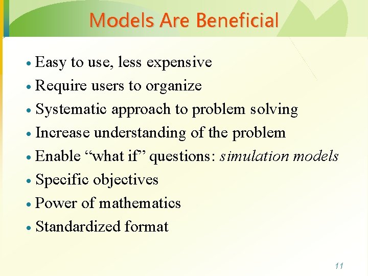
Models Are Beneficial Easy to use, less expensive · Require users to organize · Systematic approach to problem solving · Increase understanding of the problem · Enable “what if” questions: simulation models · Specific objectives · Power of mathematics · Standardized format · 11

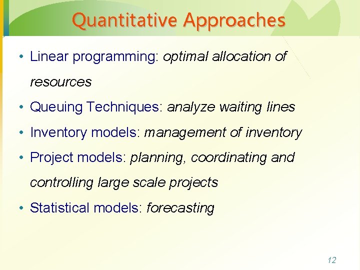
Quantitative Approaches • Linear programming: optimal allocation of resources • Queuing Techniques: analyze waiting lines • Inventory models: management of inventory • Project models: planning, coordinating and controlling large scale projects • Statistical models: forecasting 12

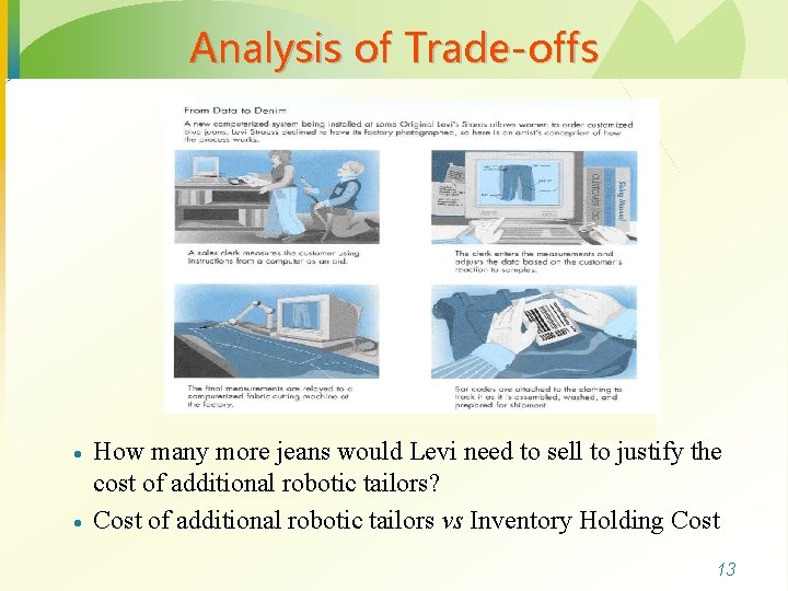
Analysis of Trade-offs · · How many more jeans would Levi need to sell to justify the cost of additional robotic tailors? Cost of additional robotic tailors vs Inventory Holding Cost 13

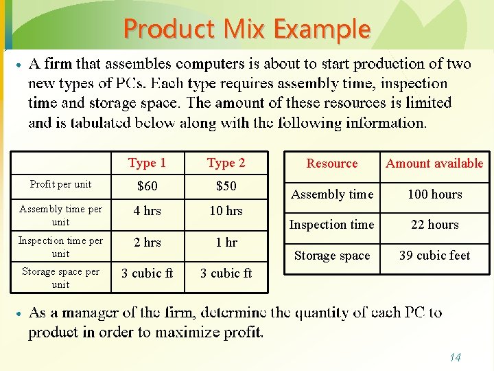
Product Mix Example Type 1 Type 2 Profit per unit $60 $50 Assembly time per unit 4 hrs 10 hrs Inspection time per unit 2 hrs 1 hr Storage space per unit 3 cubic ft Resource Amount available Assembly time 100 hours Inspection time 22 hours Storage space 39 cubic feet 14

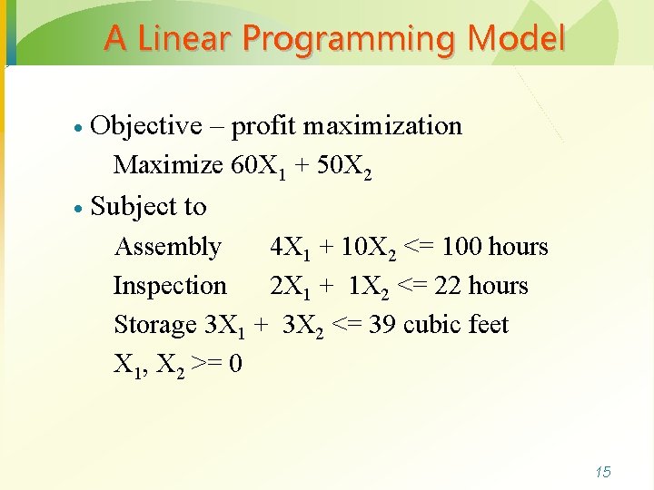
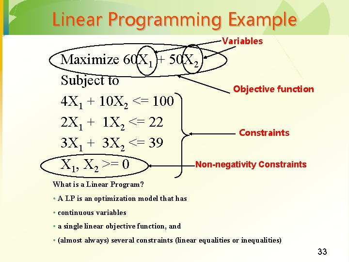
A Linear Programming Model · Objective – profit maximization Maximize 60 X 1 + 50 X 2 · Subject to Assembly 4 X 1 + 10 X 2 <= 100 hours Inspection 2 X 1 + 1 X 2 <= 22 hours Storage 3 X 1 + 3 X 2 <= 39 cubic feet X 1, X 2 >= 0 15

Cost, Revenue and Profit Models 16

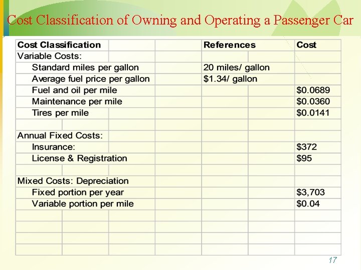
Cost Classification of Owning and Operating a Passenger Car 17

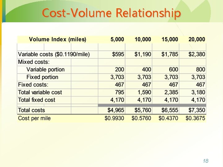
Cost-Volume Relationship 18

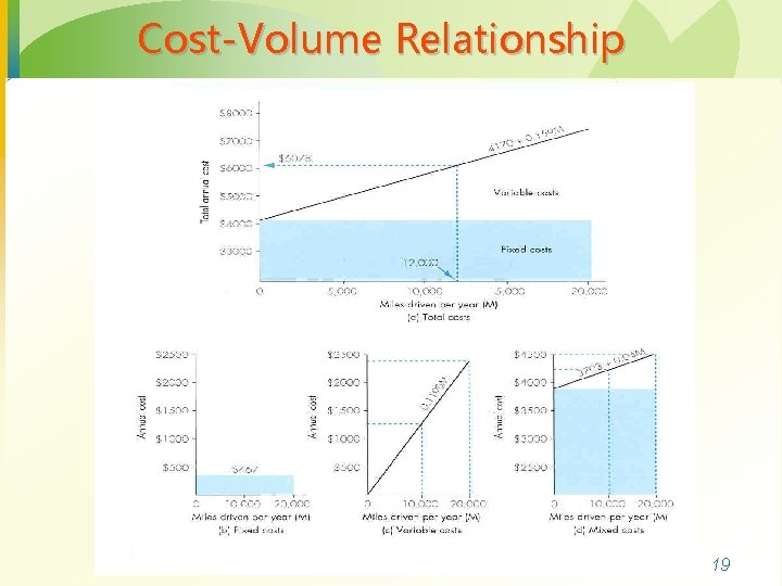
Cost-Volume Relationship 19

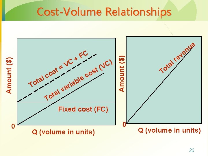
lc ota T t s o C V = ta o T ) C t (V s o c e l b ia r a lv C F + Amount ($) Cost-Volume Relationships e u en ev r l a t o T Fixed cost (FC) 0 Q (volume in units) 20

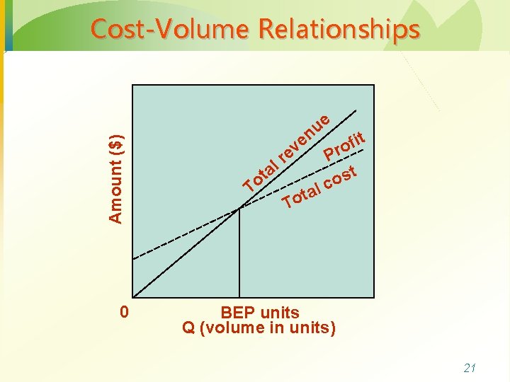
Amount ($) Cost-Volume Relationships 0 ve a t o T e u n e r l t i f ro P st o c l a ot T BEP units Q (volume in units) 21

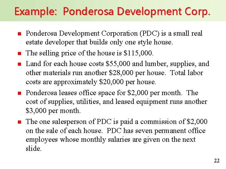
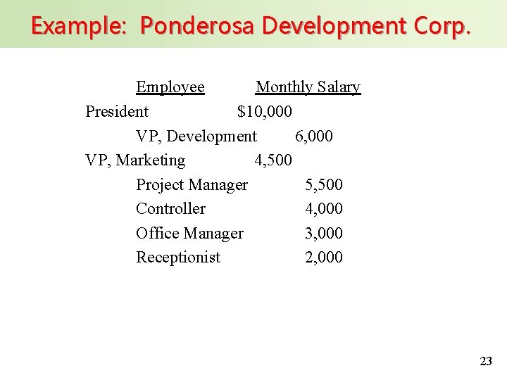
Example: Ponderosa Development Corp. n n n Ponderosa Development Corporation (PDC) is a small real estate developer that builds only one style house. The selling price of the house is $115, 000. Land for each house costs $55, 000 and lumber, supplies, and other materials run another $28, 000 per house. Total labor costs are approximately $20, 000 per house. Ponderosa leases office space for $2, 000 per month. The cost of supplies, utilities, and leased equipment runs another $3, 000 per month. The one salesperson of PDC is paid a commission of $2, 000 on the sale of each house. PDC has seven permanent office employees whose monthly salaries are given on the next slide. 22

Example: Ponderosa Development Corp. Employee Monthly Salary President $10, 000 VP, Development 6, 000 VP, Marketing 4, 500 Project Manager 5, 500 Controller 4, 000 Office Manager 3, 000 Receptionist 2, 000 23

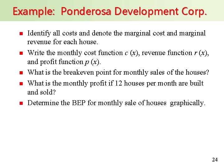
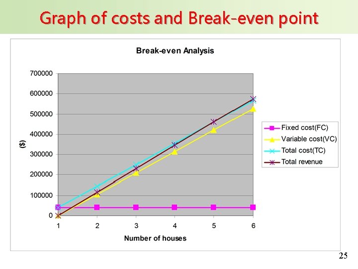
Example: Ponderosa Development Corp. n n n Identify all costs and denote the marginal cost and marginal revenue for each house. Write the monthly cost function c (x), revenue function r (x), and profit function p (x). What is the breakeven point for monthly sales of the houses? What is the monthly profit if 12 houses per month are built and sold? Determine the BEP for monthly sale of houses graphically. 24

Graph of costs and Break-even point 25

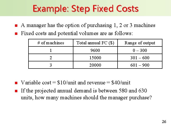
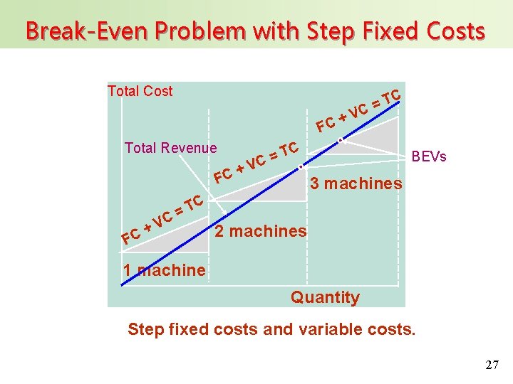
Example: Step Fixed Costs n n A manager has the option of purchasing 1, 2 or 3 machines Fixed costs and potential volumes are as follows: # of machines Total annual FC ($) Range of output 1 9600 0 – 300 2 15000 301 – 600 3 20000 601 – 900 Variable cost = $10/unit and revenue = $40/unit If the projected annual demand is between 580 and 630 units, how many machines should the manager purchase? 26

Break-Even Problem with Step Fixed Costs Total Cost C T C= V + FC Total Revenue + FC TC = C V BEVs 3 machines C T = C F V + C 2 machines 1 machine Quantity Step fixed costs and variable costs. 27

Assumptions of Cost-Volume Analysis 1. One product is involved 2. Everything produced can be sold 3. Variable cost per unit is the same regardless of volume 4. Fixed costs do not change with volume 5. Revenue per unit constant with volume 6. Revenue per unit exceeds variable cost per unit 28

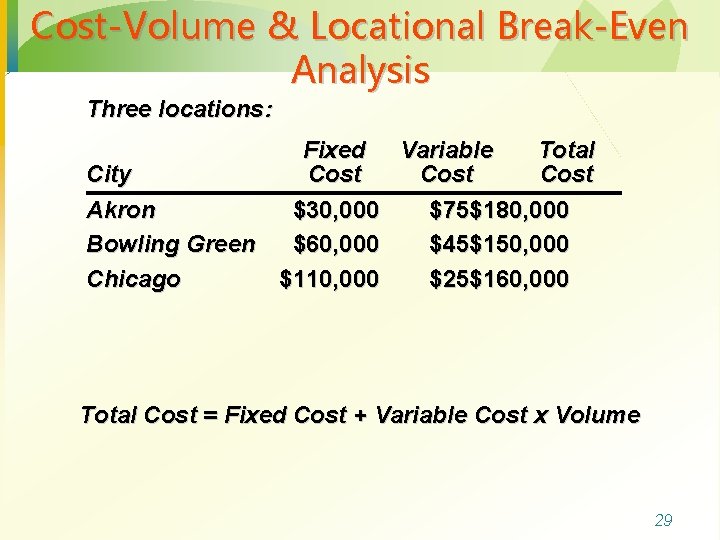
Cost-Volume & Locational Break-Even Analysis Three locations: Fixed Variable Total City Cost Akron $30, 000 $75$180, 000 Bowling Green $60, 000 $45$150, 000 Chicago $110, 000 $25$160, 000 Total Cost = Fixed Cost + Variable Cost x Volume 29

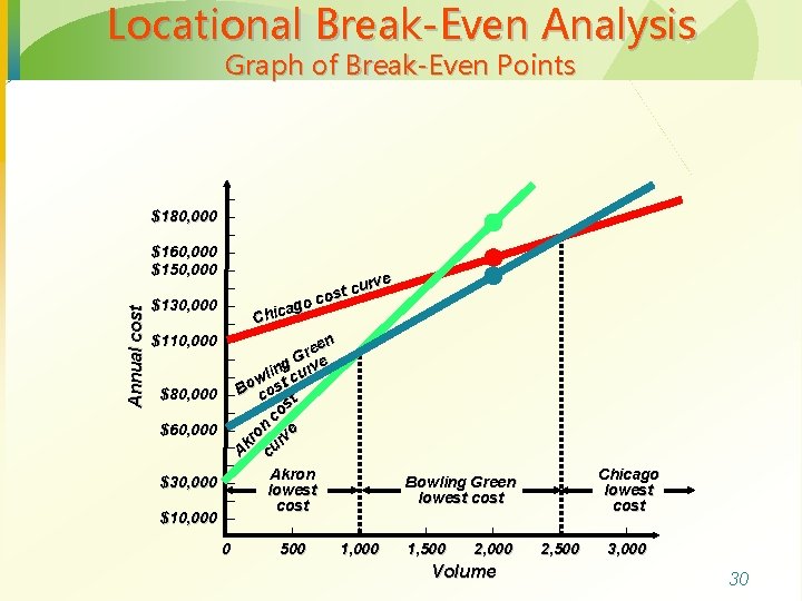
Locational Break-Even Analysis Annual cost Graph of Break-Even Points – $180, 000 – – $160, 000 – $150, 000 – urve – c t s o co $130, 000 – g a ic – Ch $110, 000 – n ee r – g G rve n i – wl t cu o $80, 000 – B cos t s – co n $60, 000 – ro rve k – A cu – Akron Bowling Green $30, 000 – lowest cost – cost $10, 000 – | | | – 0 500 1, 000 1, 500 2, 000 Volume Chicago lowest cost | | 2, 500 3, 000 30

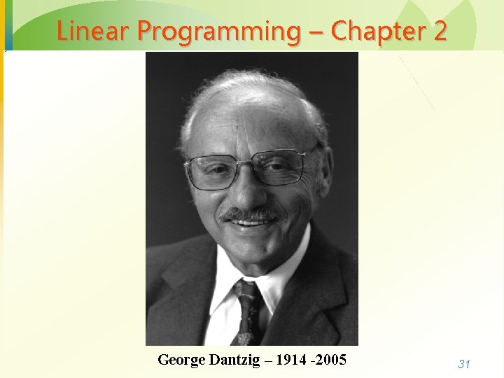
Linear Programming – Chapter 2 George Dantzig – 1914 -2005 31

Linear Programming · Concerned with optimal allocation of limited resources such as Materials · Budgets · Labor · Machine time · among competitive activities · under a set of constraints · 32

Linear Programming Example Variables Maximize 60 X 1 + 50 X 2 Subject to Objective function 4 X 1 + 10 X 2 <= 100 2 X 1 + 1 X 2 <= 22 Constraints 3 X 1 + 3 X 2 <= 39 Non-negativity Constraints X 1, X 2 >= 0 What is a Linear Program? • A LP is an optimization model that has • continuous variables • a single linear objective function, and • (almost always) several constraints (linear equalities or inequalities) 33

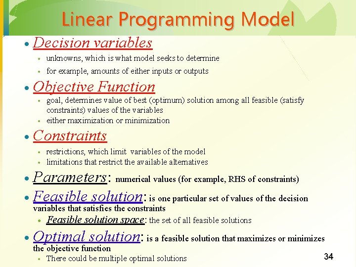
Linear Programming Model · Decision variables · · · Objective Function · · · unknowns, which is what model seeks to determine for example, amounts of either inputs or outputs goal, determines value of best (optimum) solution among all feasible (satisfy constraints) values of the variables either maximization or minimization Constraints · · restrictions, which limit variables of the model limitations that restrict the available alternatives Parameters: numerical values (for example, RHS of constraints) · Feasible solution: is one particular set of values of the decision · variables that satisfies the constraints · · Feasible solution space: the set of all feasible solutions Optimal solution: is a feasible solution that maximizes or minimizes the objective function · There could be multiple optimal solutions 34

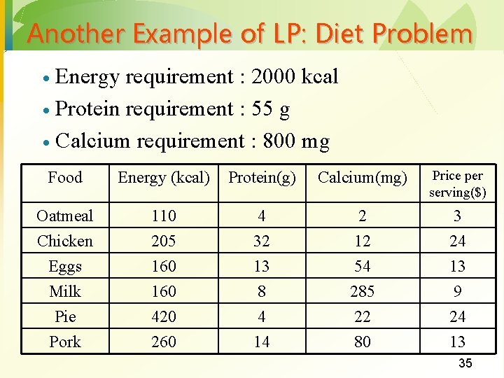
Another Example of LP: Diet Problem Energy requirement : 2000 kcal · Protein requirement : 55 g · Calcium requirement : 800 mg · Food Energy (kcal) Protein(g) Calcium(mg) Price per serving($) Oatmeal Chicken Eggs Milk Pie 110 205 160 420 4 32 13 8 4 2 12 54 285 22 3 24 13 9 24 Pork 260 14 80 13 35

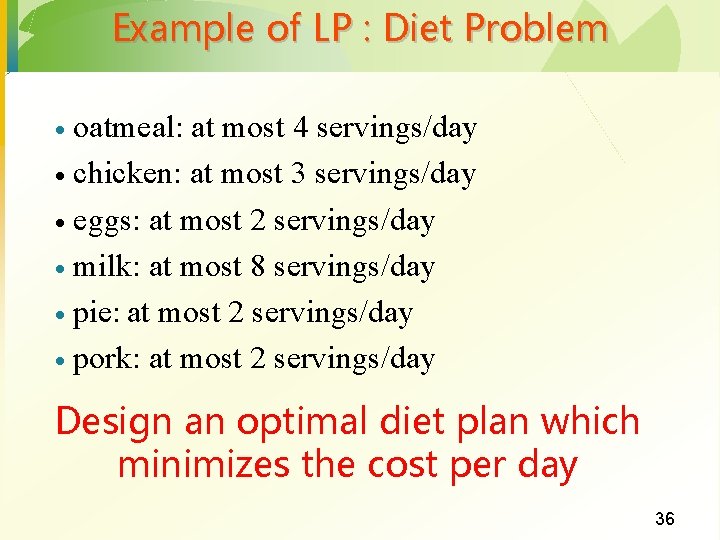
Example of LP : Diet Problem oatmeal: at most 4 servings/day · chicken: at most 3 servings/day · eggs: at most 2 servings/day · milk: at most 8 servings/day · pie: at most 2 servings/day · pork: at most 2 servings/day · Design an optimal diet plan which minimizes the cost per day 36

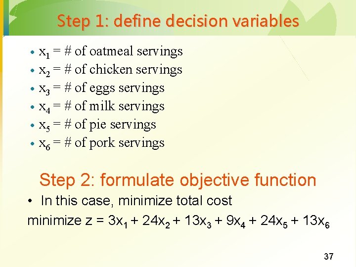
Step 1: define decision variables · · · x 1 = # of oatmeal servings x 2 = # of chicken servings x 3 = # of eggs servings x 4 = # of milk servings x 5 = # of pie servings x 6 = # of pork servings Step 2: formulate objective function • In this case, minimize total cost minimize z = 3 x 1 + 24 x 2 + 13 x 3 + 9 x 4 + 24 x 5 + 13 x 6 37

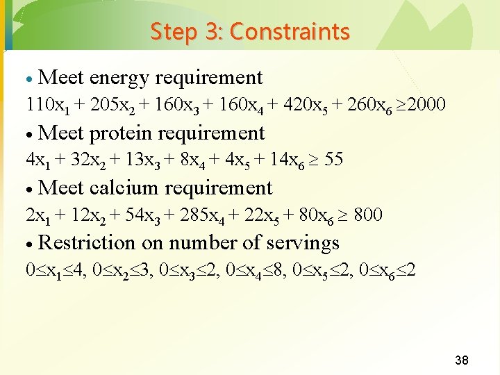
Step 3: Constraints · Meet energy requirement 110 x 1 + 205 x 2 + 160 x 3 + 160 x 4 + 420 x 5 + 260 x 6 2000 · Meet protein requirement 4 x 1 + 32 x 2 + 13 x 3 + 8 x 4 + 4 x 5 + 14 x 6 55 · Meet calcium requirement 2 x 1 + 12 x 2 + 54 x 3 + 285 x 4 + 22 x 5 + 80 x 6 800 · Restriction on number of servings 0 x 1 4, 0 x 2 3, 0 x 3 2, 0 x 4 8, 0 x 5 2, 0 x 6 2 38

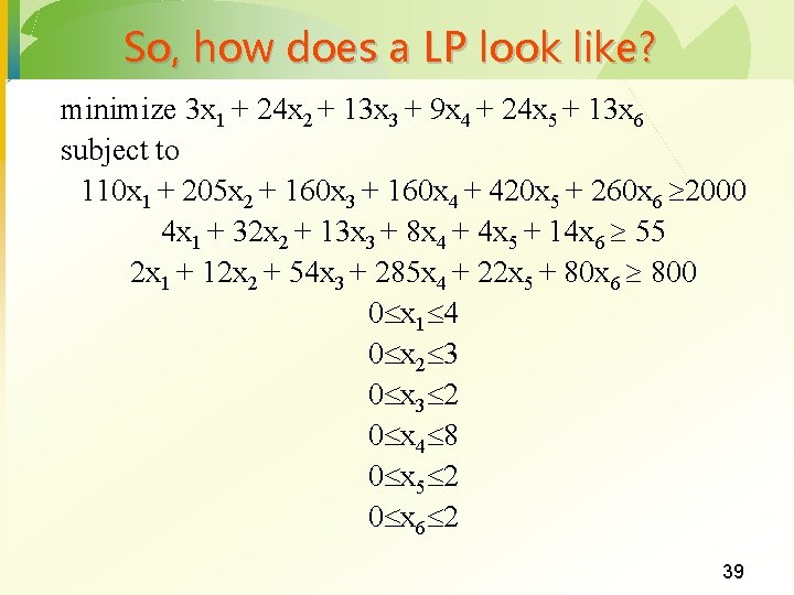
So, how does a LP look like? minimize 3 x 1 + 24 x 2 + 13 x 3 + 9 x 4 + 24 x 5 + 13 x 6 subject to 110 x 1 + 205 x 2 + 160 x 3 + 160 x 4 + 420 x 5 + 260 x 6 2000 4 x 1 + 32 x 2 + 13 x 3 + 8 x 4 + 4 x 5 + 14 x 6 55 2 x 1 + 12 x 2 + 54 x 3 + 285 x 4 + 22 x 5 + 80 x 6 800 0 x 1 4 0 x 2 3 0 x 3 2 0 x 4 8 0 x 5 2 0 x 6 2 39

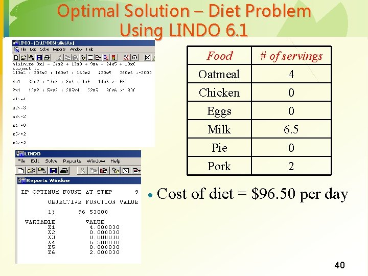
Optimal Solution – Diet Problem Using LINDO 6. 1 Food Oatmeal Chicken Eggs Milk Pie Pork · # of servings 4 0 0 6. 5 0 2 Cost of diet = $96. 50 per day 40

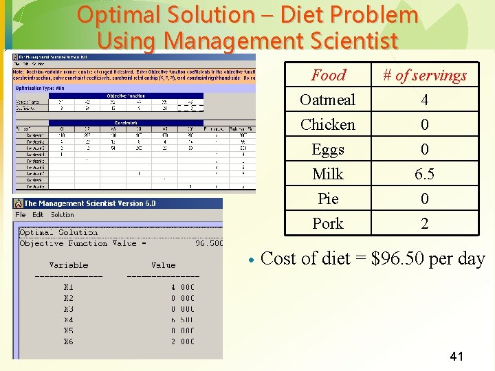
Optimal Solution – Diet Problem Using Management Scientist Food Oatmeal Chicken Eggs Milk Pie Pork · # of servings 4 0 0 6. 5 0 2 Cost of diet = $96. 50 per day 41

Guidelines for Model Formulation Understand the problem thoroughly. · Describe the objective. · Describe each constraint. · Define the decision variables. · Write the objective in terms of the decision variables. · Write the constraints in terms of the decision variables · · Do not forget non-negativity constraints 42

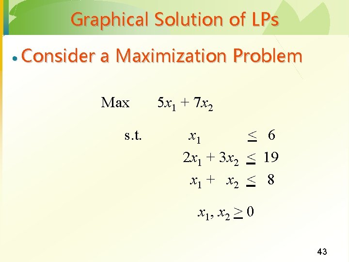
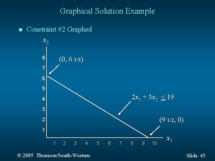
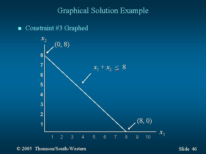
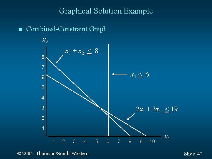
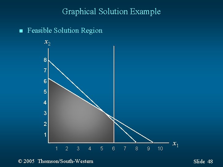
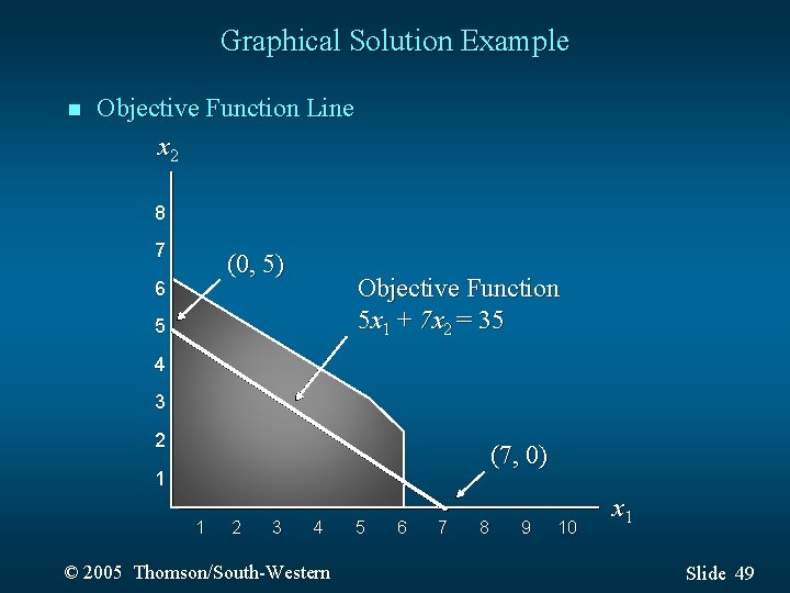
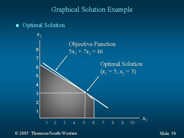
Graphical Solution of LPs · Consider a Maximization Problem Max s. t. 5 x 1 + 7 x 2 x 1 < 6 2 x 1 + 3 x 2 < 19 x 1 + x 2 < 8 x 1, x 2 > 0 43

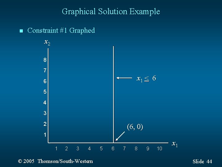
Graphical Solution Example n Constraint #1 Graphed x 2 8 7 x 1 < 6 6 5 4 3 2 (6, 0) 1 1 2 3 4 © 2005 Thomson/South-Western 5 6 7 8 9 10 x 1 Slide 44

Graphical Solution Example n Constraint #2 Graphed x 2 8 (0, 6 1/3) 7 6 5 2 x 1 + 3 x 2 < 19 4 3 (9 1/2, 0) 2 1 1 2 3 4 © 2005 Thomson/South-Western 5 6 7 8 9 10 x 1 Slide 45

Graphical Solution Example n Constraint #3 Graphed x 2 (0, 8) 8 7 x 1 + x 2 < 8 6 5 4 3 2 (8, 0) 1 1 2 3 4 © 2005 Thomson/South-Western 5 6 7 8 9 10 x 1 Slide 46

Graphical Solution Example n Combined-Constraint Graph x 2 x 1 + x 2 < 8 8 7 x 1 < 6 6 5 4 3 2 x 1 + 3 x 2 < 19 2 1 1 2 3 4 © 2005 Thomson/South-Western 5 6 7 8 9 10 x 1 Slide 47

Graphical Solution Example n Feasible Solution Region x 2 8 7 6 5 4 3 Feasible Region 2 1 1 2 3 4 © 2005 Thomson/South-Western 5 6 7 8 9 10 x 1 Slide 48

Graphical Solution Example n Objective Function Line x 2 8 7 (0, 5) 6 Objective Function 5 x 1 + 7 x 2 = 35 5 4 3 2 (7, 0) 1 1 2 3 4 © 2005 Thomson/South-Western 5 6 7 8 9 10 x 1 Slide 49

Graphical Solution Example n Optimal Solution x 2 Objective Function 5 x 1 + 7 x 2 = 46 8 7 Optimal Solution (x 1 = 5, x 2 = 3) 6 5 4 3 2 1 1 2 3 4 © 2005 Thomson/South-Western 5 6 7 8 9 10 x 1 Slide 50

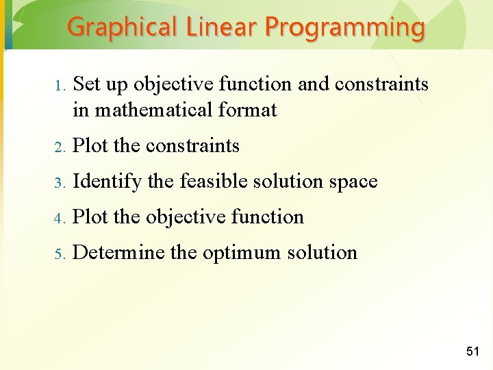
Graphical Linear Programming 1. Set up objective function and constraints in mathematical format 2. Plot the constraints 3. Identify the feasible solution space 4. Plot the objective function 5. Determine the optimum solution 51

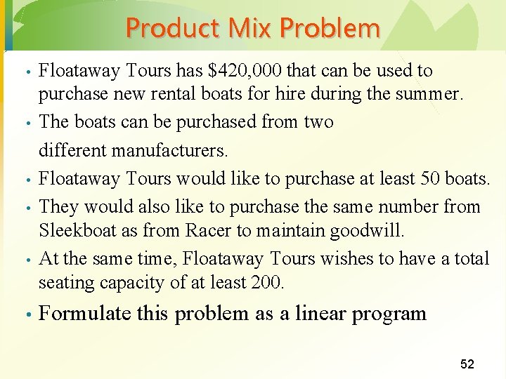
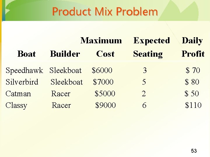
Product Mix Problem • • • Floataway Tours has $420, 000 that can be used to purchase new rental boats for hire during the summer. The boats can be purchased from two different manufacturers. Floataway Tours would like to purchase at least 50 boats. They would also like to purchase the same number from Sleekboat as from Racer to maintain goodwill. At the same time, Floataway Tours wishes to have a total seating capacity of at least 200. Formulate this problem as a linear program 52

Product Mix Problem Boat Maximum Builder Cost Speedhawk Sleekboat Silverbird Sleekboat Catman Racer Classy Racer $6000 $7000 $5000 $9000 Expected Seating 3 5 2 6 Daily Profit $ 70 $ 80 $ 50 $110 53

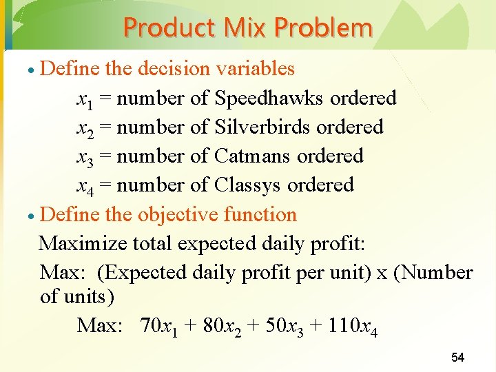
Product Mix Problem Define the decision variables x 1 = number of Speedhawks ordered x 2 = number of Silverbirds ordered x 3 = number of Catmans ordered x 4 = number of Classys ordered · Define the objective function Maximize total expected daily profit: Max: (Expected daily profit per unit) x (Number of units) Max: 70 x 1 + 80 x 2 + 50 x 3 + 110 x 4 · 54

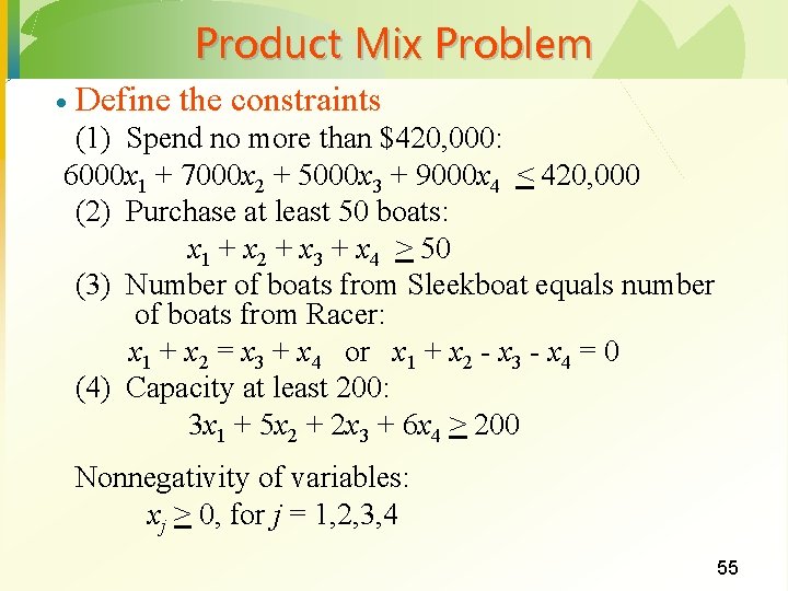
Product Mix Problem · Define the constraints (1) Spend no more than $420, 000: 6000 x 1 + 7000 x 2 + 5000 x 3 + 9000 x 4 < 420, 000 (2) Purchase at least 50 boats: x 1 + x 2 + x 3 + x 4 > 50 (3) Number of boats from Sleekboat equals number of boats from Racer: x 1 + x 2 = x 3 + x 4 or x 1 + x 2 - x 3 - x 4 = 0 (4) Capacity at least 200: 3 x 1 + 5 x 2 + 2 x 3 + 6 x 4 > 200 Nonnegativity of variables: xj > 0, for j = 1, 2, 3, 4 55

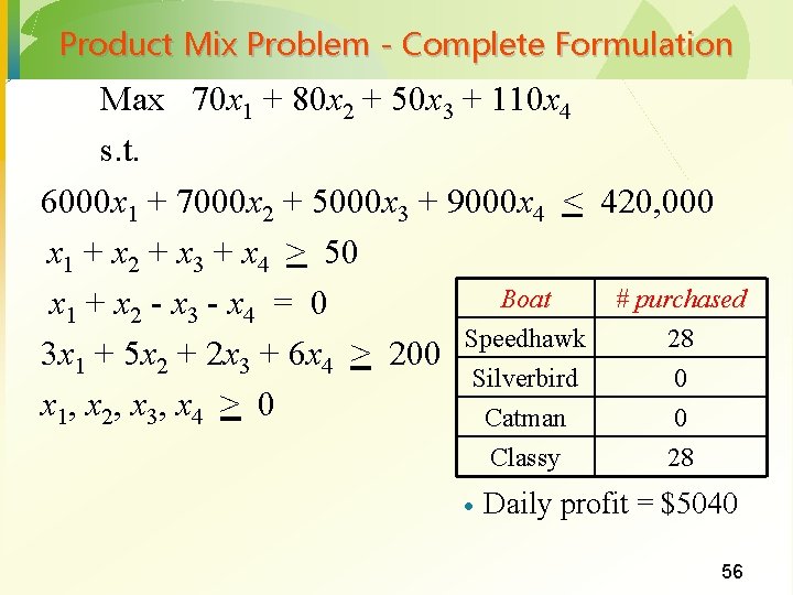
Product Mix Problem - Complete Formulation Max 70 x 1 + 80 x 2 + 50 x 3 + 110 x 4 s. t. 6000 x 1 + 7000 x 2 + 5000 x 3 + 9000 x 4 < 420, 000 x 1 + x 2 + x 3 + x 4 > 50 Boat # purchased x 1 + x 2 - x 3 - x 4 = 0 Speedhawk 28 3 x 1 + 5 x 2 + 2 x 3 + 6 x 4 > 200 Silverbird 0 x 1, x 2, x 3, x 4 > 0 Catman 0 Classy · 28 Daily profit = $5040 56

Applications of LP Product mix planning · Distribution networks · Truck routing · Staff scheduling · Financial portfolios · Capacity planning · Media selection: marketing · 57