Lecture 4 MGMT 650 Network Models Shortest Path

Lecture 4 MGMT 650 Network Models – Shortest Path Project Scheduling Forecasting

Shortest Path Problem · · Belongs to class of problems typically known as network flow models What is the “best way” to traverse a network to get from one point to another as cheaply as possible? Network consists of nodes and arcs For example, consider a transportation network · · Nodes represent cities Arcs represent travel distances between cities Criterion to be minimized in the shortest path problem not limited to distance Other criteria include time and cost 2

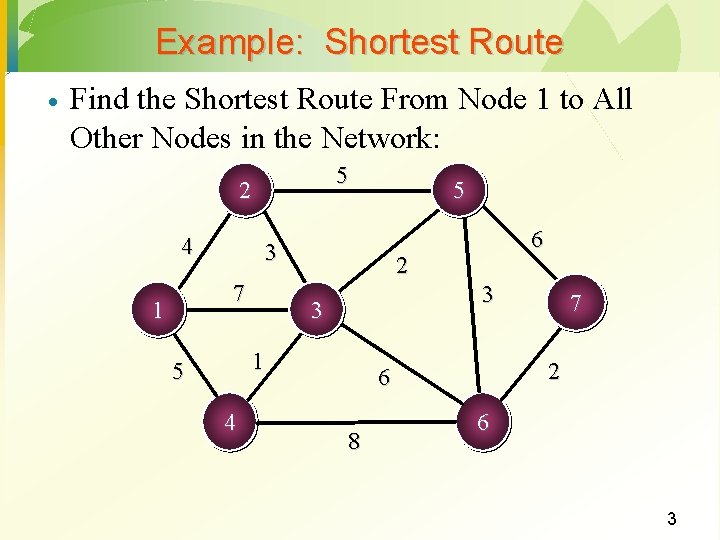
Example: Shortest Route · Find the Shortest Route From Node 1 to All Other Nodes in the Network: 5 2 4 3 7 1 5 2 3 3 1 5 4 6 2 6 8 7 6 3

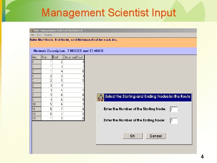
Management Scientist Input 4

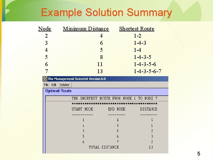
Example Solution Summary Node 2 3 4 5 6 7 Minimum Distance 4 6 5 8 11 13 Shortest Route 1 -2 1 -4 -3 -5 1 -4 -3 -5 -6 -7 5

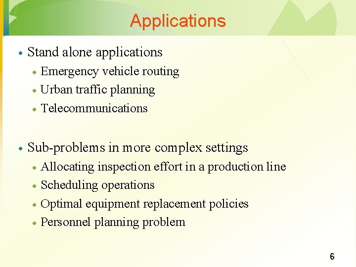
Applications · Stand alone applications · · Emergency vehicle routing Urban traffic planning Telecommunications Sub-problems in more complex settings · · Allocating inspection effort in a production line Scheduling operations Optimal equipment replacement policies Personnel planning problem 6

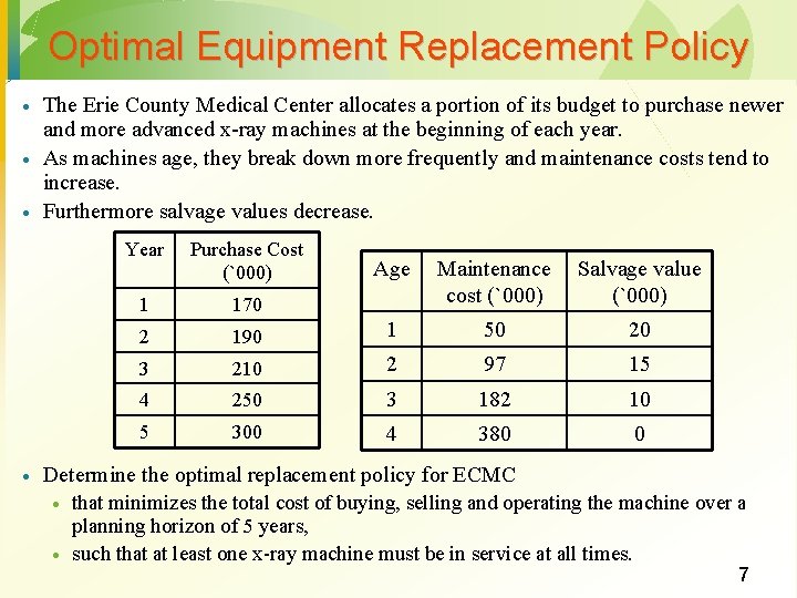
Optimal Equipment Replacement Policy · · The Erie County Medical Center allocates a portion of its budget to purchase newer and more advanced x-ray machines at the beginning of each year. As machines age, they break down more frequently and maintenance costs tend to increase. Furthermore salvage values decrease. Year Purchase Cost (`000) 1 170 2 Age Maintenance cost (`000) Salvage value (`000) 190 1 50 20 3 210 2 97 15 4 250 3 182 10 5 300 4 380 0 Determine the optimal replacement policy for ECMC · · that minimizes the total cost of buying, selling and operating the machine over a planning horizon of 5 years, such that at least one x-ray machine must be in service at all times. 7

Lecture 4 Project Scheduling Chapter 10

Project Management · How is it different? Limited time frame · Narrow focus, specific objectives · · Why is it used? Special needs · Pressures for new or improves products or services · · Definition of a project · Unique, one-time sequence of activities designed to accomplish a specific set of objectives in a limited time frame 9

Project Scheduling: PERT/CPM Project Scheduling with Known Activity Times · Project Scheduling with Uncertain Activity Times · 10

PERT/CPM · PERT · · CPM · · Program Evaluation and Review Technique Critical Path Method PERT and CPM have been used to plan, schedule, and control a wide variety of projects: R&D of new products and processes · Construction of buildings and highways · Maintenance of large and complex equipment · Design and installation of new systems · 11

PERT/CPM is used to plan the scheduling of individual activities that make up a project. · Projects may have as many as several thousand activities. · A complicating factor in carrying out the activities is that some activities depend on the completion of other activities before they can be started. · 12

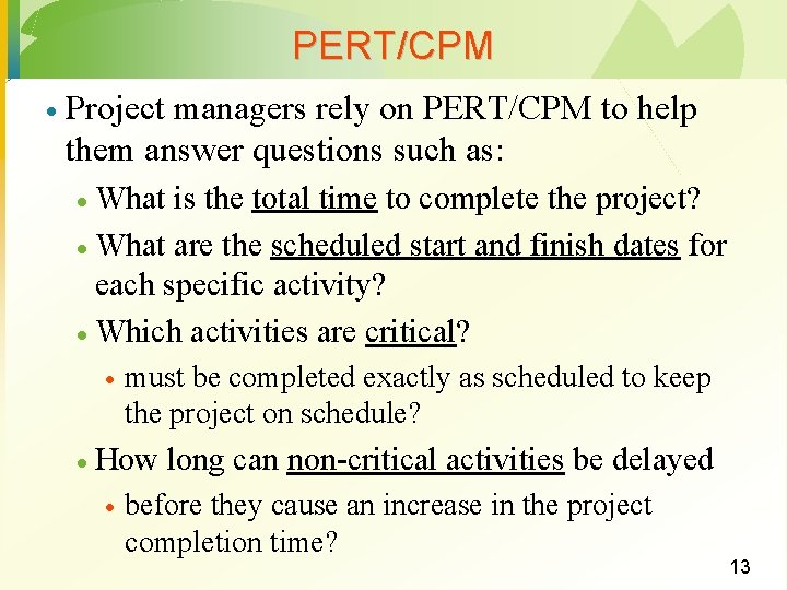
PERT/CPM · Project managers rely on PERT/CPM to help them answer questions such as: What is the total time to complete the project? · What are the scheduled start and finish dates for each specific activity? · Which activities are critical? · · · must be completed exactly as scheduled to keep the project on schedule? How long can non-critical activities be delayed · before they cause an increase in the project completion time? 13

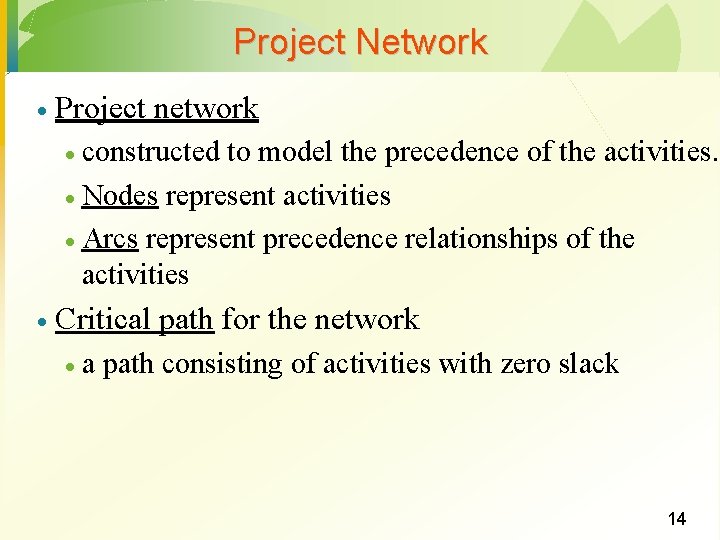
Project Network · Project network constructed to model the precedence of the activities. · Nodes represent activities · Arcs represent precedence relationships of the activities · · Critical path for the network · a path consisting of activities with zero slack 14

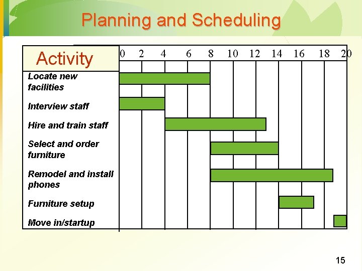
Planning and Scheduling Activity 0 2 4 6 8 10 12 14 16 18 20 Locate new facilities Interview staff Hire and train staff Select and order furniture Remodel and install phones Furniture setup Move in/startup 15

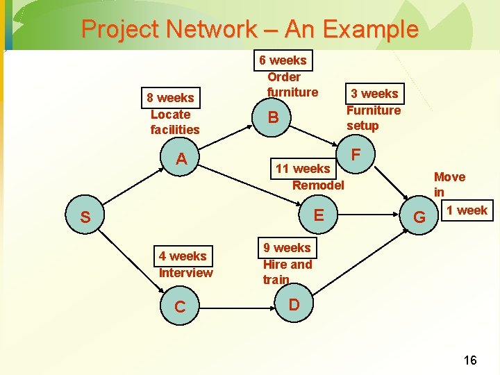
Project Network – An Example 8 weeks Locate facilities A 6 weeks Order furniture B 11 weeks Remodel E S 4 weeks Interview C 3 weeks Furniture setup F G Move in 1 week 9 weeks Hire and train D 16

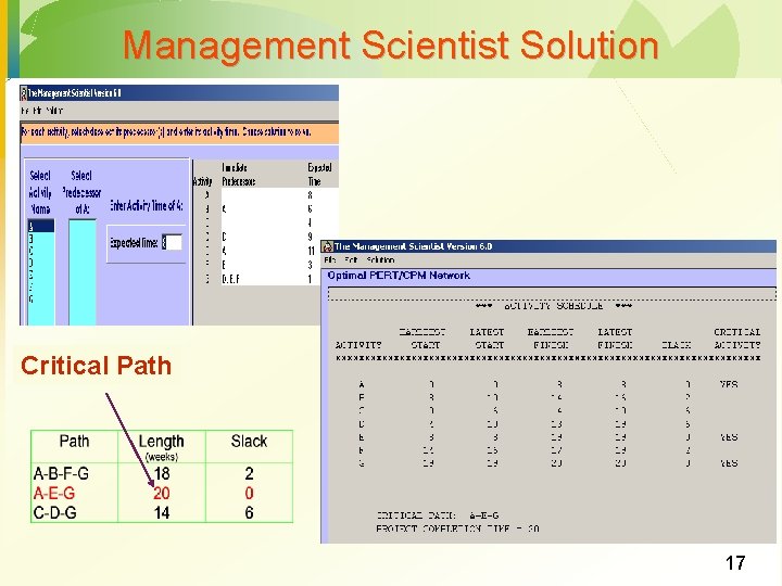
Management Scientist Solution Critical Path 17

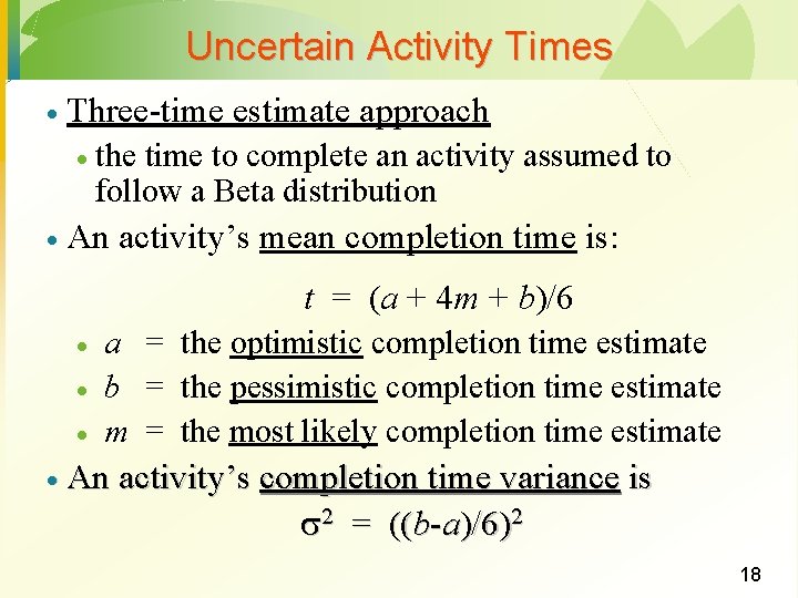
Uncertain Activity Times · Three-time estimate approach · · the time to complete an activity assumed to follow a Beta distribution An activity’s mean completion time is: t = (a + 4 m + b)/6 · · · a = the optimistic completion time estimate b = the pessimistic completion time estimate m = the most likely completion time estimate · An activity’s completion time variance is 2 = ((b-a)/6)2 18

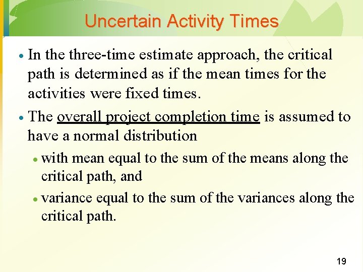
Uncertain Activity Times In the three-time estimate approach, the critical path is determined as if the mean times for the activities were fixed times. · The overall project completion time is assumed to have a normal distribution · with mean equal to the sum of the means along the critical path, and · variance equal to the sum of the variances along the critical path. · 19

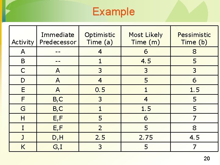
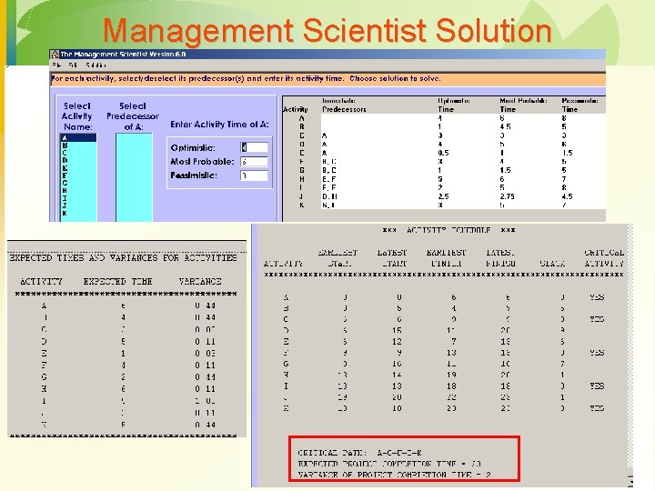
Example Immediate Activity Predecessor Optimistic Time (a) Most Likely Time (m) Pessimistic Time (b) A -- 4 6 8 B -- 1 4. 5 5 C A 3 3 3 D A 4 5 6 E A 0. 5 1 1. 5 F B, C 3 4 5 G B, C 1 1. 5 5 H E, F 5 6 7 I E, F 2 5 8 J D, H 2. 5 2. 75 4. 5 K G, I 3 5 7 20

Management Scientist Solution 21

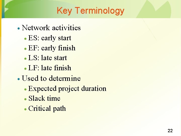
Key Terminology · Network activities ES: early start · EF: early finish · LS: late start · LF: late finish · · Used to determine Expected project duration · Slack time · Critical path · 22

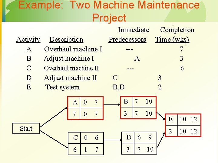
Example: Two Machine Maintenance Project Immediate Completion Activity Description Predecessors Time (wks) A Overhaul machine I --7 B Adjust machine I A 3 C Overhaul machine II --6 D Adjust machine II C 3 E Test system B, D 2 A 0 7 B 7 10 7 7 3 10 0 7 Start C 0 6 D 6 6 7 3 1 9 7 10 E 10 12 2 10 12

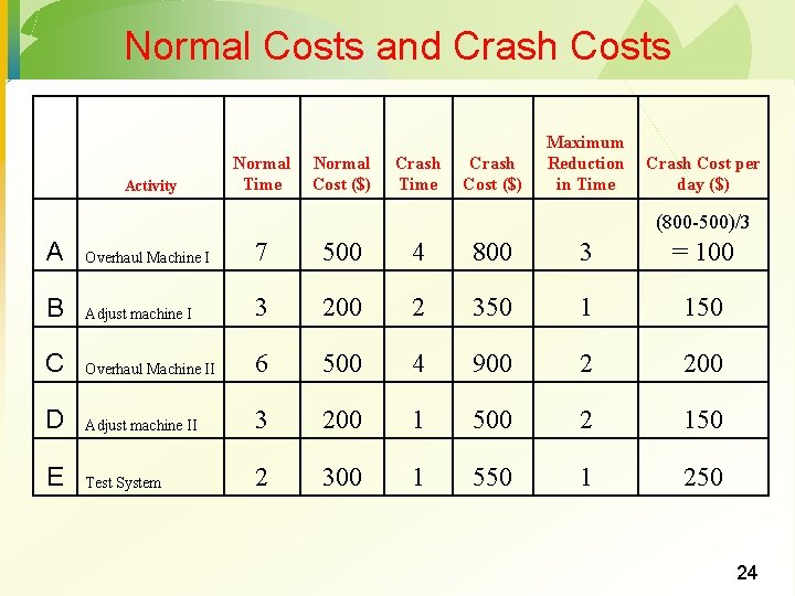
Normal Costs and Crash Costs Activity Normal Time Normal Cost ($) Crash Time Crash Cost ($) Maximum Reduction in Time Crash Cost per day ($) (800 -500)/3 A Overhaul Machine I 7 500 4 800 3 = 100 B Adjust machine I 3 200 2 350 1 150 C Overhaul Machine II 6 500 4 900 2 200 D Adjust machine II 3 200 1 500 2 150 E Test System 2 300 1 550 1 250 24

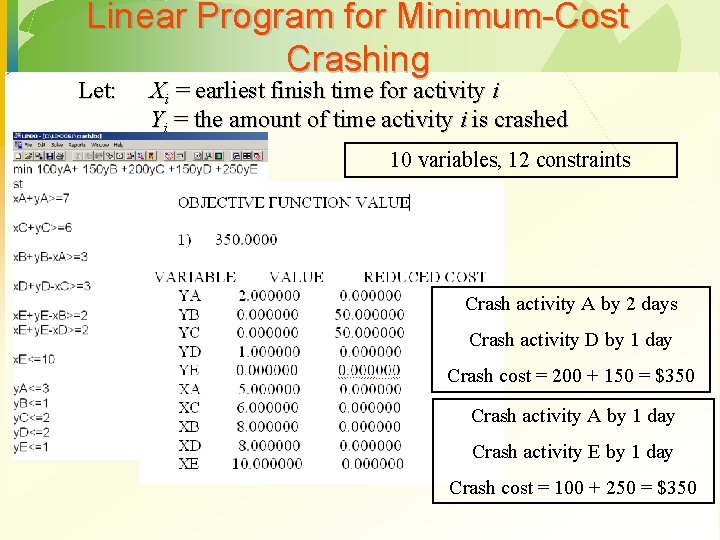
Linear Program for Minimum-Cost Crashing Let: Xi = earliest finish time for activity i Yi = the amount of time activity i is crashed 10 variables, 12 constraints Crash activity A by 2 days Crash activity D by 1 day Crash cost = 200 + 150 = $350 Crash activity A by 1 day Crash activity E by 1 day Crash cost = 100 + 250 = $350

Lecture 4 Forecasting Chapter 16

Forecasting - Topics · Quantitative Approaches to Forecasting · The Components of a Time Series · Measures of Forecast Accuracy · Using Smoothing Methods in Forecasting · Using Trend Projection in Forecasting 27

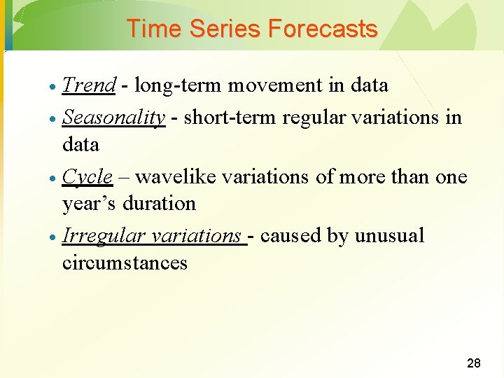
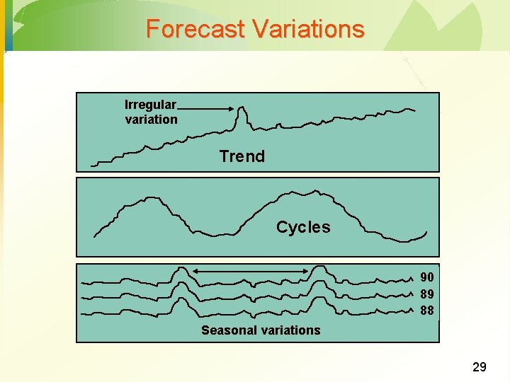
Time Series Forecasts Trend - long-term movement in data · Seasonality - short-term regular variations in data · Cycle – wavelike variations of more than one year’s duration · Irregular variations - caused by unusual circumstances · 28

Forecast Variations Irregular variation Trend Cycles 90 89 88 Seasonal variations 29

Smoothing/Averaging Methods Used in cases in which the time series is fairly stable and has no significant trend, seasonal, or cyclical effects · Purpose of averaging - to smooth out the irregular components of the time series. · Four common smoothing/averaging methods are: · Moving averages · Weighted moving averages · Exponential smoothing · 30

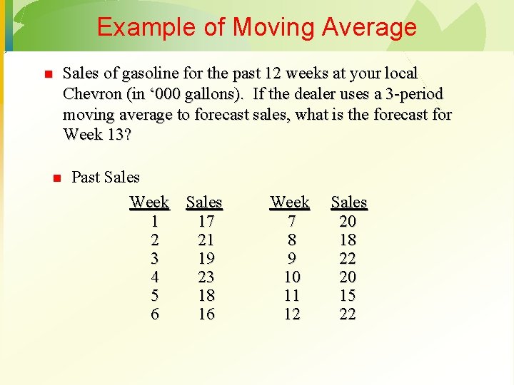
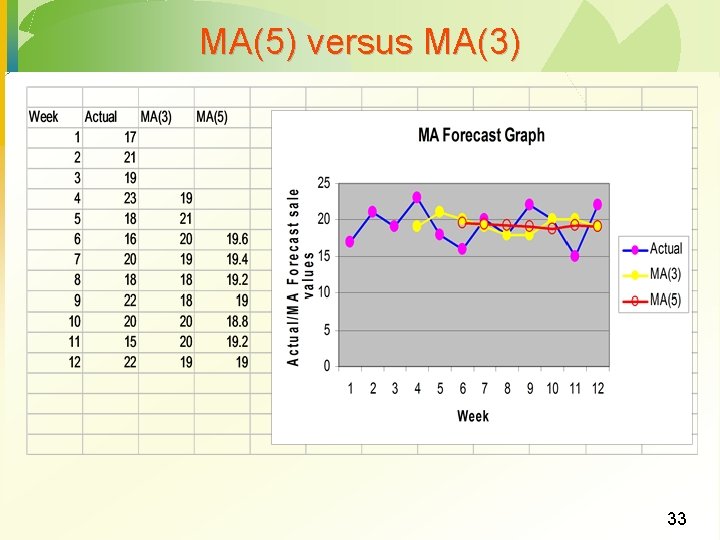
Example of Moving Average n n Sales of gasoline for the past 12 weeks at your local Chevron (in ‘ 000 gallons). If the dealer uses a 3 -period moving average to forecast sales, what is the forecast for Week 13? Past Sales Week Sales 1 17 2 21 3 19 4 23 5 18 6 16 Week 7 8 9 10 11 12 Sales 20 18 22 20 15 22

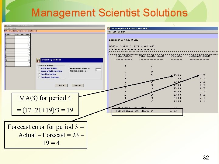
Management Scientist Solutions MA(3) for period 4 = (17+21+19)/3 = 19 Forecast error for period 3 = Actual – Forecast = 23 – 19 = 4 32

MA(5) versus MA(3) 33

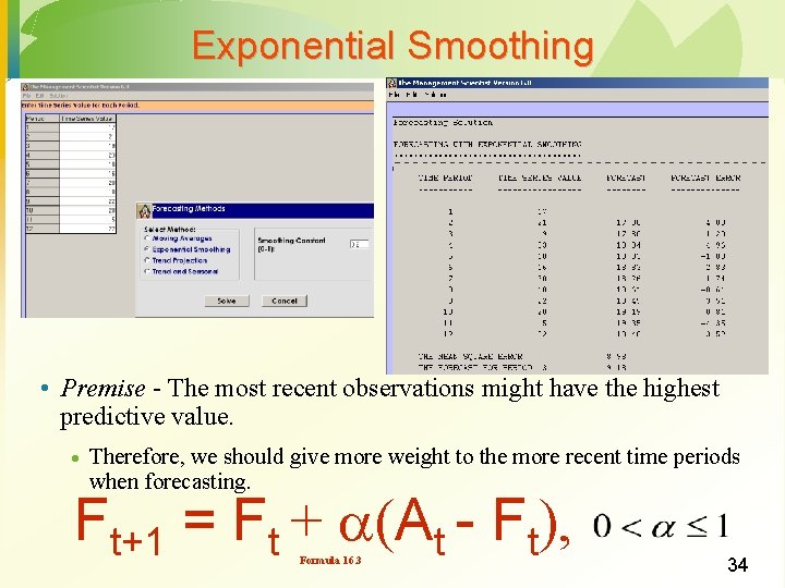
Exponential Smoothing • Premise - The most recent observations might have the highest predictive value. · Therefore, we should give more weight to the more recent time periods when forecasting. Ft+1 = Ft + (At - Ft), Formula 16. 3 34

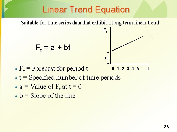
Linear Trend Equation Suitable for time series data that exhibit a long term linear trend Ft Ft = a + bt a · · 0 1 2 Ft = Forecast for period t t = Specified number of time periods a = Value of Ft at t = 0 b = Slope of the line 3 4 5 t 35

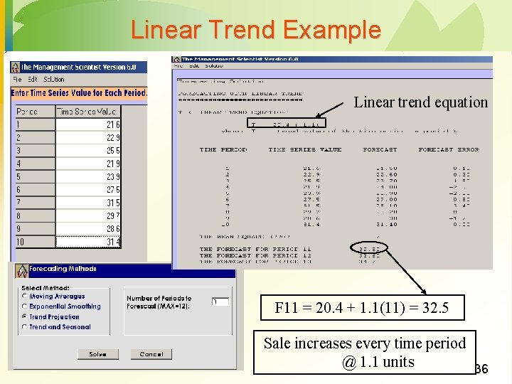
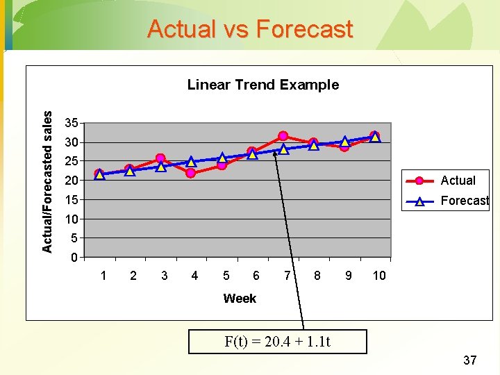
Linear Trend Example Linear trend equation F 11 = 20. 4 + 1. 1(11) = 32. 5 Sale increases every time period @ 1. 1 units 36

Actual vs Forecast Actual/Forecasted sales Linear Trend Example 35 30 25 20 Actual 15 Forecast 10 5 0 1 2 3 4 5 6 7 8 9 10 Week F(t) = 20. 4 + 1. 1 t 37

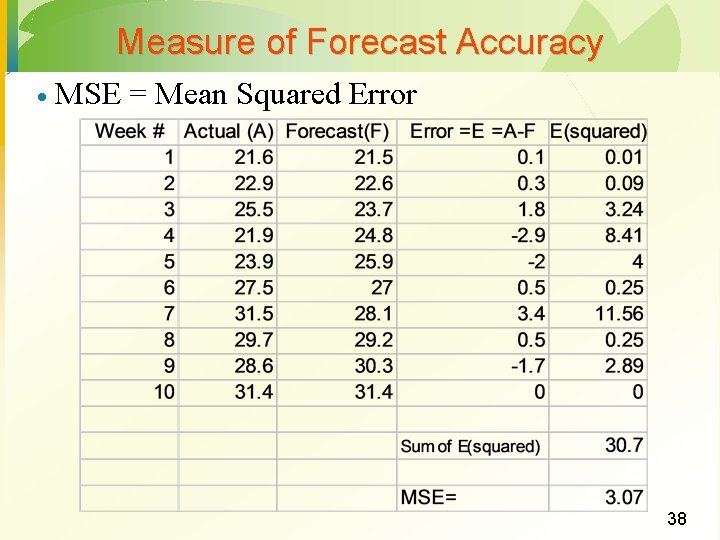
Measure of Forecast Accuracy · MSE = Mean Squared Error 38

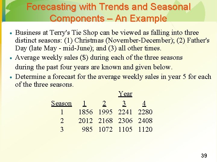
Forecasting with Trends and Seasonal Components – An Example · · · Business at Terry's Tie Shop can be viewed as falling into three distinct seasons: (1) Christmas (November-December); (2) Father's Day (late May - mid-June); and (3) all other times. Average weekly sales ($) during each of the three seasons during the past four years are known and given below. Determine a forecast for the average weekly sales in year 5 for each of the three seasons. Year Season 1 2 3 4 1 1856 1995 2241 2280 2 2012 2168 2306 2408 3 985 1072 1105 1120 39

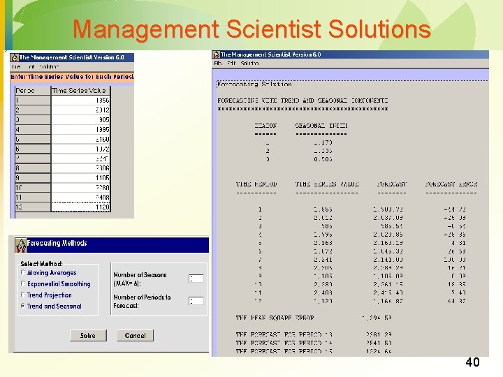
Management Scientist Solutions 40

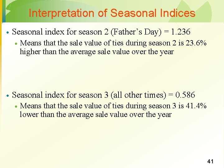
Interpretation of Seasonal Indices · Seasonal index for season 2 (Father’s Day) = 1. 236 · · Means that the sale value of ties during season 2 is 23. 6% higher than the average sale value over the year Seasonal index for season 3 (all other times) = 0. 586 · Means that the sale value of ties during season 3 is 41. 4% lower than the average sale value over the year 41