Graph Algorithms with Map Reduce Chapter 5 Thanks

Graph Algorithms with Map. Reduce Chapter 5 Thanks to Jimmy Lin slides

Topics • Introduction to graph algorithms and graph representations • Single Source Shortest Path (SSSP) problem – Refresher: Dijkstra’s algorithm – Breadth-First Search with Map. Reduce • Page. Rank

What’s a graph? • G = (V, E), where – V represents the set of vertices (nodes) – E represents the set of edges (links) – Both vertices and edges may contain additional information • Different types of graphs: – Directed vs. undirected edges – Presence or absence of cycles • Graphs are everywhere: – – Hyperlink structure of the Web Physical structure of computers on the Internet Interstate highway system Social networks

Some Graph Problems • Finding shortest paths – Routing Internet traffic and UPS trucks • Finding minimum spanning trees – Telco laying down fiber • Finding Max Flow – Airline scheduling • Identify “special” nodes and communities – Breaking up terrorist cells, spread of avian flu • Bipartite matching – Monster. com, Match. com • And of course. . . Page. Rank

Graphs and Map. Reduce • Graph algorithms typically involve: – Performing computation at each node – Processing node-specific data, edge-specific data, and link structure – Traversing the graph in some manner • Key questions: – How do you represent graph data in Map. Reduce? – How do you traverse a graph in Map. Reduce?

Representing Graphs • G = (V, E) – A poor representation for computational purposes • Two common representations – Adjacency matrix – Adjacency list

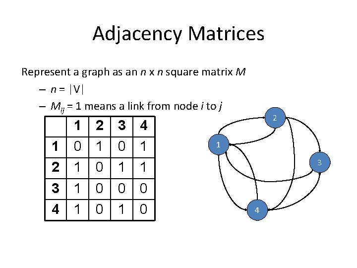
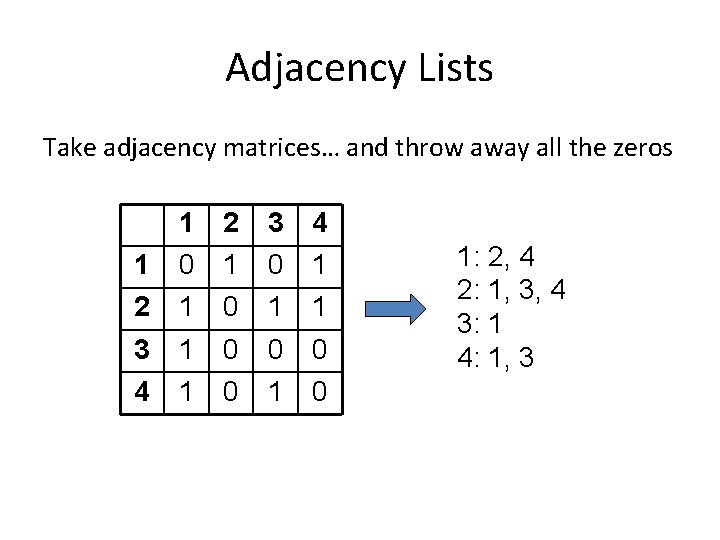
Adjacency Matrices Represent a graph as an n x n square matrix M – n = |V| – Mij = 1 means a link from node i to j 1 1 0 2 1 3 0 4 1 2 1 0 1 1 3 4 1 1 0 0 0 1 0 0 2 1 3 4

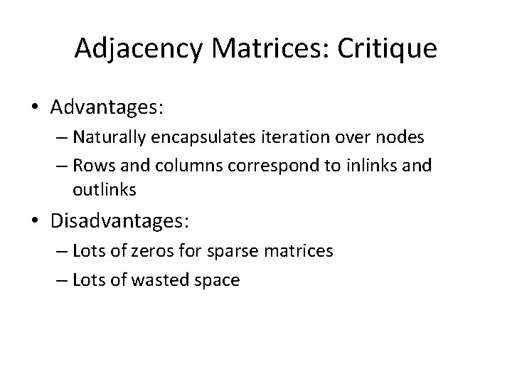
Adjacency Matrices: Critique • Advantages: – Naturally encapsulates iteration over nodes – Rows and columns correspond to inlinks and outlinks • Disadvantages: – Lots of zeros for sparse matrices – Lots of wasted space

Adjacency Lists Take adjacency matrices… and throw away all the zeros 1 1 0 2 1 3 0 4 1 2 1 0 1 1 3 4 1 1 0 0 0 1: 2, 4 2: 1, 3, 4 3: 1 4: 1, 3

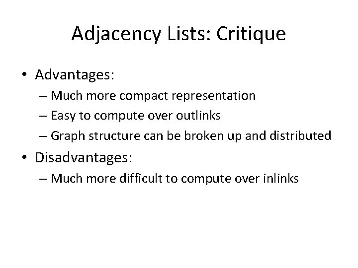
Adjacency Lists: Critique • Advantages: – Much more compact representation – Easy to compute over outlinks – Graph structure can be broken up and distributed • Disadvantages: – Much more difficult to compute over inlinks

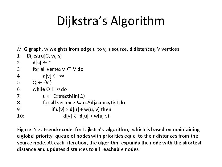
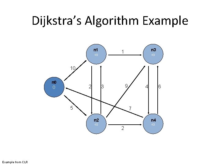
Single Source Shortest Path • Problem: find shortest path from a source node to one or more target nodes • “Graph search algorithm that solves the single -source shortest path problem for a graph with nonnegative edge path costs, producing a shortest path tree” Wikipedia • First, a refresher: Dijkstra’s algorithm – Single machine

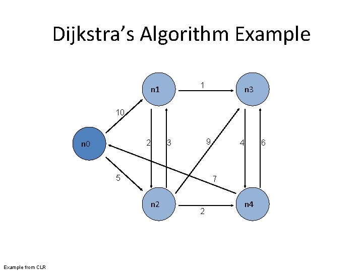
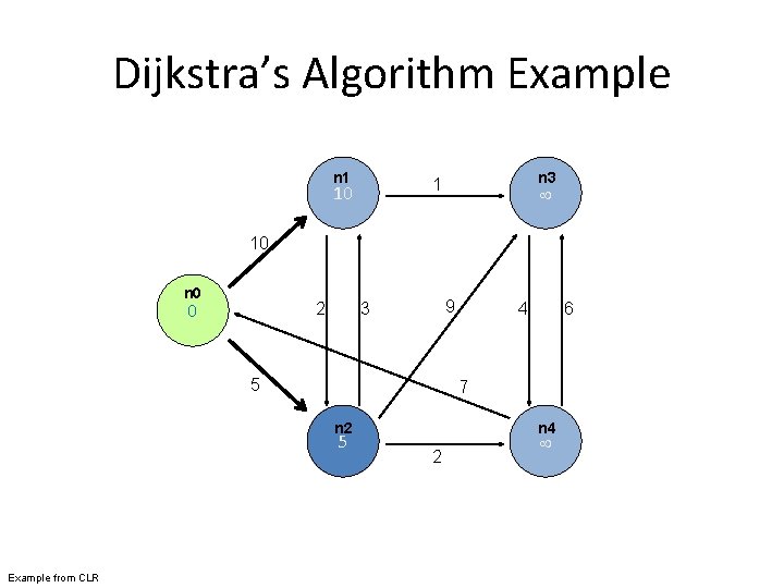
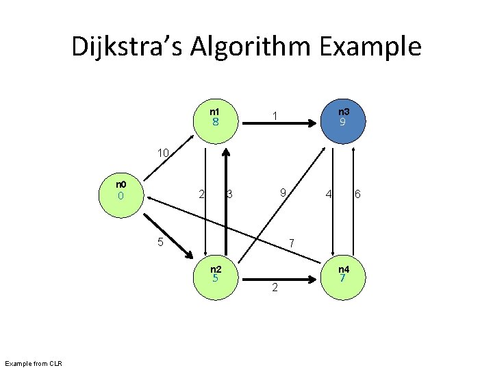
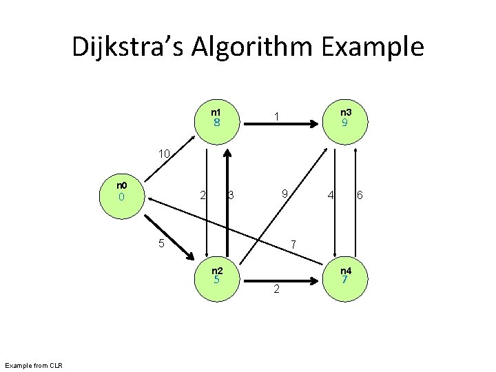
Dijkstra’s Algorithm Example 1 n 3 10 n 0 2 9 3 5 6 7 n 2 Example from CLR 4 2 n 4

Dijkstra’s Algorithm // G graph, w weights from edge u to v, s source, d distances, V vertices 1: Dijkstra(G, w, s) 2: d[s] ← 0 3: for all vertex v ∈ V do 4: d[v] ← ∞ 5: Q ← {V } 6: while Q != ∅ do 7: u ← Extract. Min(Q) 8: for all vertex v ∈ u. Adjacency. List do 9: if d[v] > d[u] + w(u, v) then 10: d[v] ← d[u] + w(u, v) Figure 5. 2: Pseudo-code for Dijkstra’s algorithm, which is based on maintaining a global priority queue of nodes with priorities equal to their distances from the source node. At each iteration, the algorithm expands the node with the shortest distance and updates distances to all reachable nodes.

Dijkstra’s Algorithm Example 1 10 0 2 9 3 5 6 7 Example from CLR 4 2

Dijkstra’s Algorithm Example n 1 n 3 1 10 n 0 0 2 9 3 5 6 7 n 2 Example from CLR 4 n 4 2

Dijkstra’s Algorithm Example n 1 n 3 1 10 10 n 0 0 2 9 3 5 6 7 n 2 5 Example from CLR 4 n 4 2

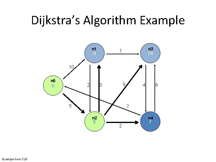
Dijkstra’s Algorithm Example n 1 n 3 1 8 14 10 n 0 0 2 9 3 5 6 7 n 2 5 Example from CLR 4 n 4 2 7

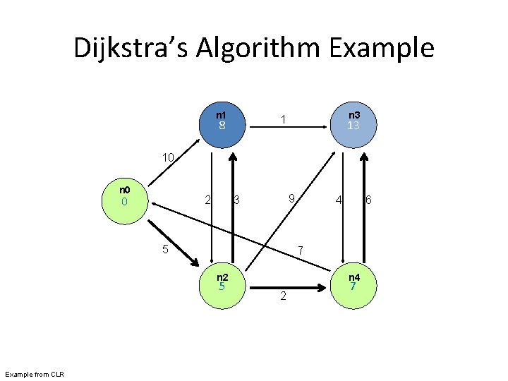
Dijkstra’s Algorithm Example n 1 n 3 1 8 13 10 n 0 0 2 9 3 5 6 7 n 2 5 Example from CLR 4 n 4 2 7

Dijkstra’s Algorithm Example n 1 n 3 1 8 9 10 n 0 0 2 9 3 5 6 7 n 2 5 Example from CLR 4 n 4 2 7

Dijkstra’s Algorithm Example n 1 n 3 1 8 9 10 n 0 0 2 9 3 5 6 7 n 2 5 Example from CLR 4 n 4 2 7

Single Source Shortest Path • Problem: find shortest path from a source node to one or more target nodes • Single processor machine: Dijkstra’s Algorithm • Map. Reduce: parallel Breadth-First Search (BFS) – How to do it? First simplify the problem!!

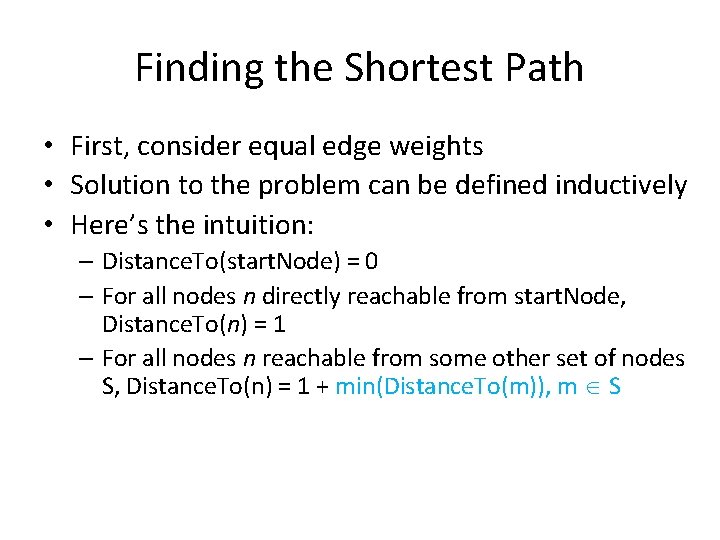
Finding the Shortest Path • First, consider equal edge weights • Solution to the problem can be defined inductively • Here’s the intuition: – Distance. To(start. Node) = 0 – For all nodes n directly reachable from start. Node, Distance. To(n) = 1 – For all nodes n reachable from some other set of nodes S, Distance. To(n) = 1 + min(Distance. To(m)), m S

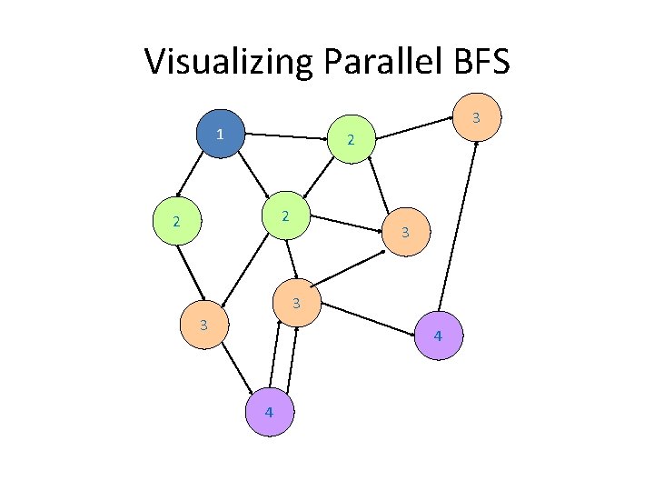
Finding the Shortest Path • This strategy advances the “known frontier” by one hop – Subsequent iterations include more reachable nodes as frontier advances – Multiple iterations are needed to explore entire graph

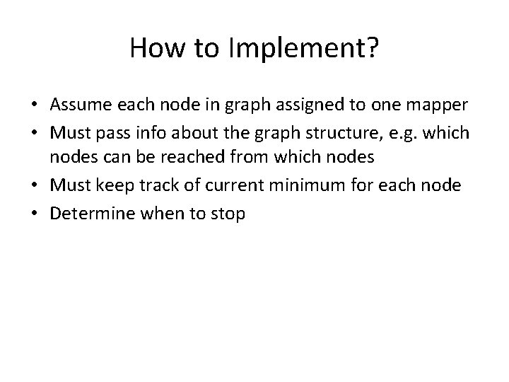
Visualizing Parallel BFS 3 1 2 2 2 3 3 3 4 4

How to Implement? • Assume each node in graph assigned to one mapper • Must pass info about the graph structure, e. g. which nodes can be reached from which nodes • Must keep track of current minimum for each node • Determine when to stop

Termination • Does the algorithm ever terminate? – Eventually, all nodes will be discovered, all edges will be considered (in a connected graph) • When do we stop? – When distances at every node no longer change at next frontier

Dijkstra’s Algorithm Example 1 n 3 10 n 0 2 9 3 5 6 7 n 2 Example from CLR 4 2 n 4

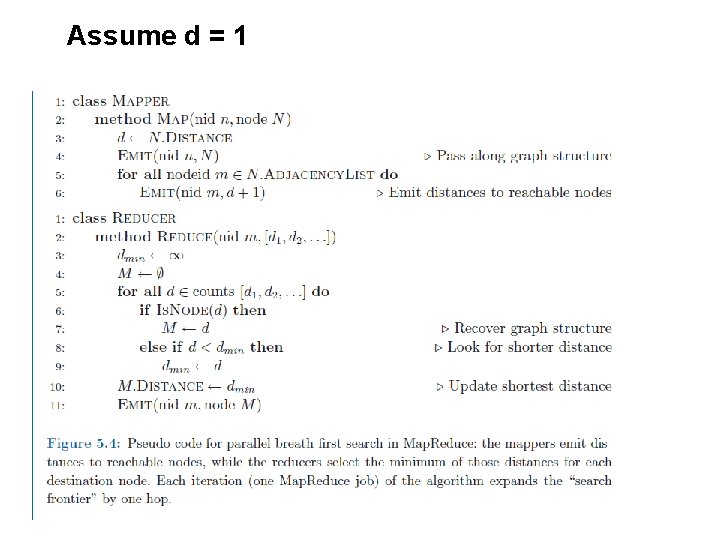
Assume d = 1

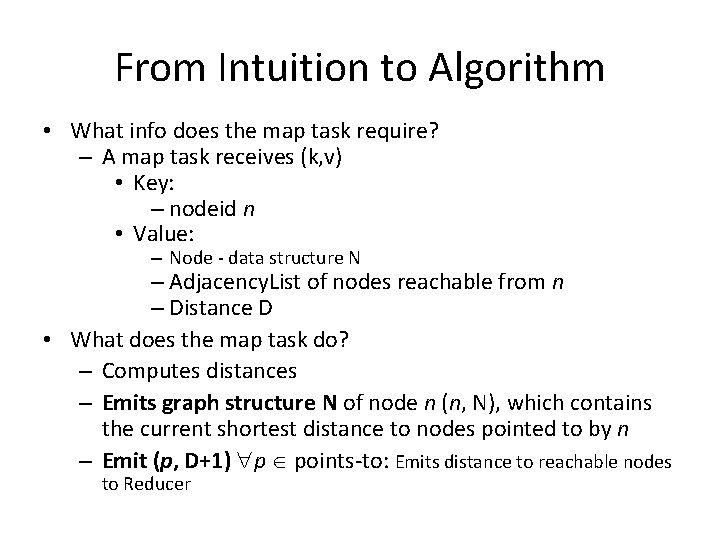
From Intuition to Algorithm • What info does the map task require? – A map task receives (k, v) • Key: – nodeid n • Value: – Node - data structure N – Adjacency. List of nodes reachable from n – Distance D • What does the map task do? – Computes distances – Emits graph structure N of node n (n, N), which contains the current shortest distance to nodes pointed to by n – Emit (p, D+1) p points-to: Emits distance to reachable nodes to Reducer

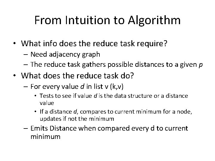
From Intuition to Algorithm • What info does the reduce task require? – Need adjacency graph – The reduce task gathers possible distances to a given p • What does the reduce task do? – For every value d in list v (k, v) • Tests to see if value d is the data structure or a distance value • If a distance d, compares to current minimum for a node, updates if not the minimum – Emits Distance when compared every d to current minimum

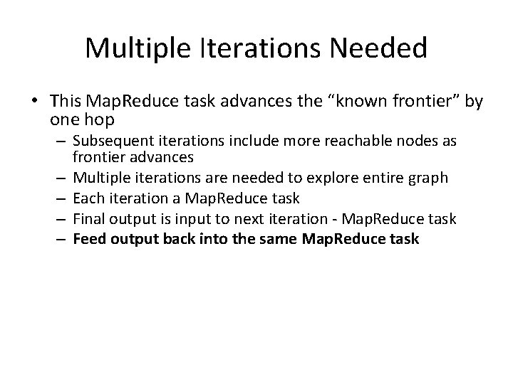
Multiple Iterations Needed • This Map. Reduce task advances the “known frontier” by one hop – Subsequent iterations include more reachable nodes as frontier advances – Multiple iterations are needed to explore entire graph – Each iteration a Map. Reduce task – Final output is input to next iteration - Map. Reduce task – Feed output back into the same Map. Reduce task

Next Step to Solving - Weighted Edges • Next – – No longer assume distance to each node is 1 – Instead of adding 1 as traverse through the graph, add the positive weights to the edges – Simple change: Include a weight w for each node p (p, D+wp) – Map Reduce emit pairs, needs a points-to-list, keep track of current minimum

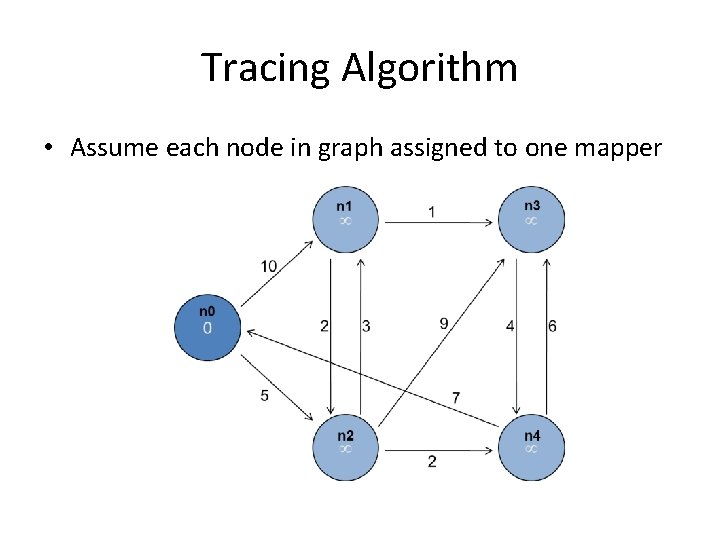
Tracing Algorithm • Assume each node in graph assigned to one mapper

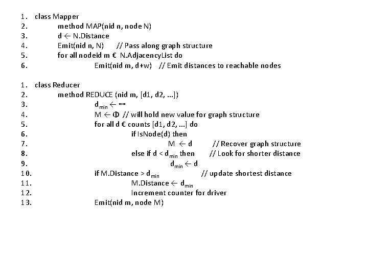
1. class Mapper 2. method MAP(nid n, node N) 3. d ← N. Distance 4. Emit(nid n, N) // Pass along graph structure 5. for all nodeid m € N. Adjacency. List do 6. Emit(nid m, d+w) // Emit distances to reachable nodes 1. class Reducer 2. method REDUCE (nid m, [d 1, d 2, . . . ]) 3. dmin ← ∞ 4. M ← Φ // will hold new value for graph structure 5. for all d € counts [d 1, d 2, . . . ] do 6. if Is. Node(d) then 7. M ←d // Recover graph structure 8. else if d < dmin then // Look for shorter distance 9. dmin ← d 10. if M. Distance > dmin // update shortest distance 11. M. Distance ← dmin 12. Increment counter for driver 13. Emit(nid m, node M)

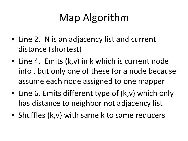
Map Algorithm • Line 2. N is an adjacency list and current distance (shortest) • Line 4. Emits (k, v) in k which is current node info , but only one of these for a node because assume each node assigned to one mapper • Line 6. Emits different type of (k, v) which only has distance to neighbor not adjacency list • Shuffles (k, v) with same k to same reducers

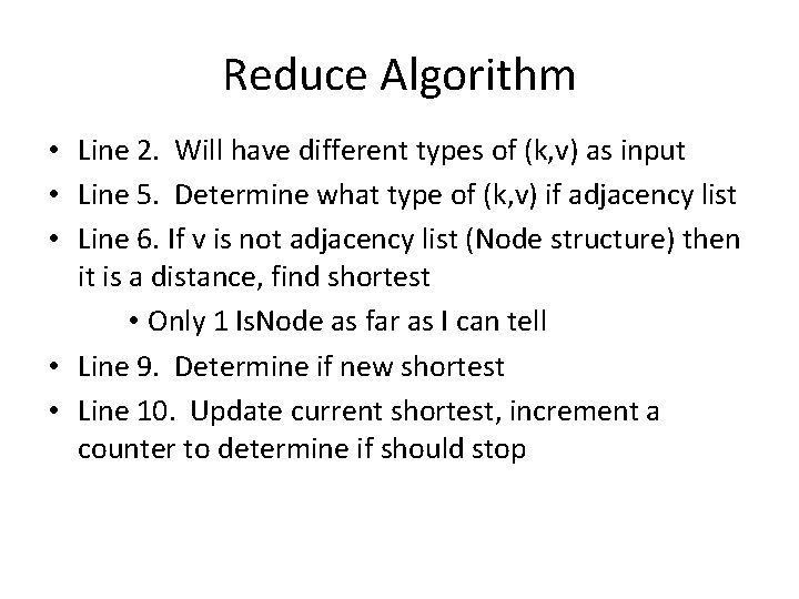
Reduce Algorithm • Line 2. Will have different types of (k, v) as input • Line 5. Determine what type of (k, v) if adjacency list • Line 6. If v is not adjacency list (Node structure) then it is a distance, find shortest • Only 1 Is. Node as far as I can tell • Line 9. Determine if new shortest • Line 10. Update current shortest, increment a counter to determine if should stop

Shortest path – one more thing • Only finds shortest distances, not the shortest path • Is this true? – Do we have to use backpointers to find shortest path to retrace – NO -– Emit paths along with distances, each node has shortest path accessible at all times • Most paths relatively short, uses little space

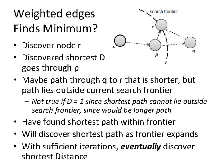
Weighted edges Finds Minimum? • Discover node r • Discovered shortest D to p and shortest D to r goes through p • Maybe path through q to r that is shorter, but path lies outside current search frontier – Not true if D = 1 since shortest path cannot lie outside search frontier, since would be longer path • Have found shortest path within frontier • Will discover shortest path as frontier expands • With sufficient iterations, eventually discover shortest Distance

Termination • Does this ever terminate? – Yes! Eventually, no better distances will be found. When distance is the same, we stop – Checking of termination must occur outside of Map. Reduce – Driver program submits MR job to iterate algorithm, see if termination condition met – Hadoop provides Counters (drivers) outside Map. Reduce • Drivers determine after reducers if done • In shortest path reducers count each change to min distance, passes count to driver

Iterations • How many iterations needed to compute shortest distance to all nodes? – Diameter of graph or greatest distance between any pair of nodes – Small for many real-world problems – 6 degrees of separation • For global social network – 6 Map. Reduce iterations

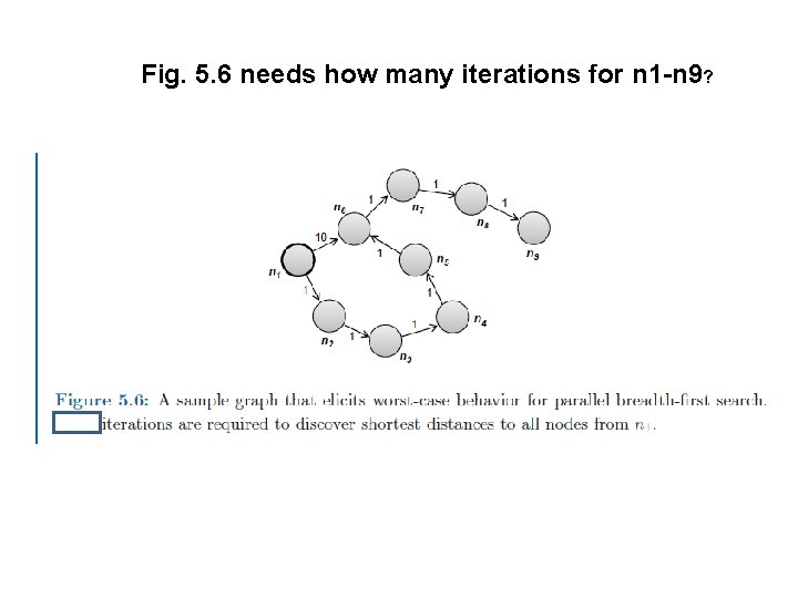
Fig. 5. 6 needs how many iterations for n 1 -n 9?

Fig. 5. 6 needs how many iterations for n 1 -n 9? • Trace through it • Worst case? • Need: #nodes – 1 – Best case?

General Approach • Map. Reduce is adept at manipulating graphs – Store graphs as adjacency lists • Graph algorithms with Map. Reduce: – Each map task receives a node and its outlinks – Map task compute some function of the link structure, emits value with target as the key – Reduce task collects keys (target nodes) and aggregates • Iterate multiple Map. Reduce cycles until some termination condition – Remember to “pass” graph structure from one iteration to next

Comparison to Dijkstra • Dijkstra versus Map. Reduce • Dijkstra’s algorithm is more efficient – At any step it only pursues edges from the minimumcost path inside the frontier • Map. Reduce explores all paths in parallel – Brute force – wastes time – Divide and conquer – Except at search frontier, within frontier repeating same computations – Throw more hardware at the problem

Another example – Random Walks Over the Web • Model: – User starts at a random Web page – User randomly clicks on links, surfing from page to page (may also teleport to completely different page) • How frequently will a page be encountered during this surfing? • This is Page. Rank – Probability distribution over nodes in a graph representing likelihood random walk over a graph will arrive at a particular node

• What characteristics would you use to rank the pages?

• For a given node n – Assign a value to node(s) m pointing to n • How many pages does m point to? • What is its current value?

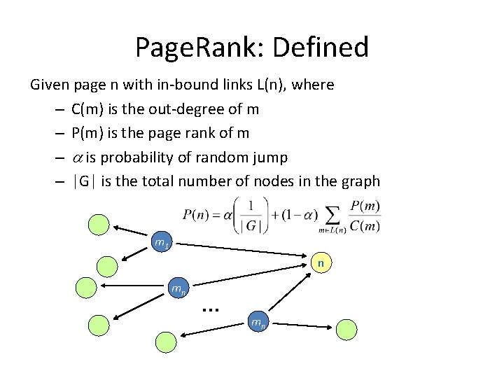
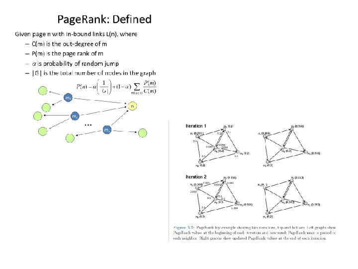
Page. Rank: Defined Given page n with in-bound links L(n), where – C(m) is the out-degree of m – P(m) is the page rank of m – is probability of random jump – |G| is the total number of nodes in the graph m 1 n mn … mn

Computing Page. Rank • Properties of Page. Rank – Can be computed iteratively – Effects at each iteration is local • Sketch of algorithm: – Start with seed (Pi ) values – Each page distributes (Pi ) “credit” to all pages it links to – Each target page adds up “credit” from multiple inbound links to compute (Pi+1) – Iterate until values converge

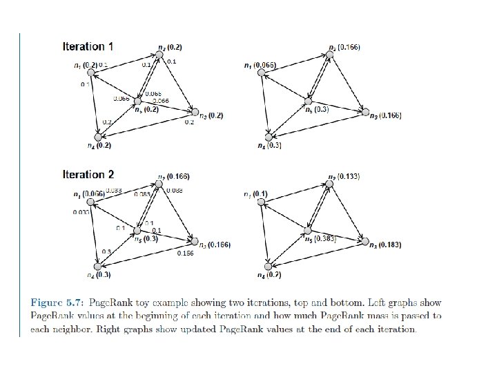
Page. Rank • Assume alpha=0 • Begins with 5 nodes splitting 1. 0 -> 0. 2 each • Add up value of inbound links to get next value

• How to implement this NOT using Map. Reduce?

Computing Page. Rank • Now implement using Map. Reduce • What does map do? • What does reduce do?

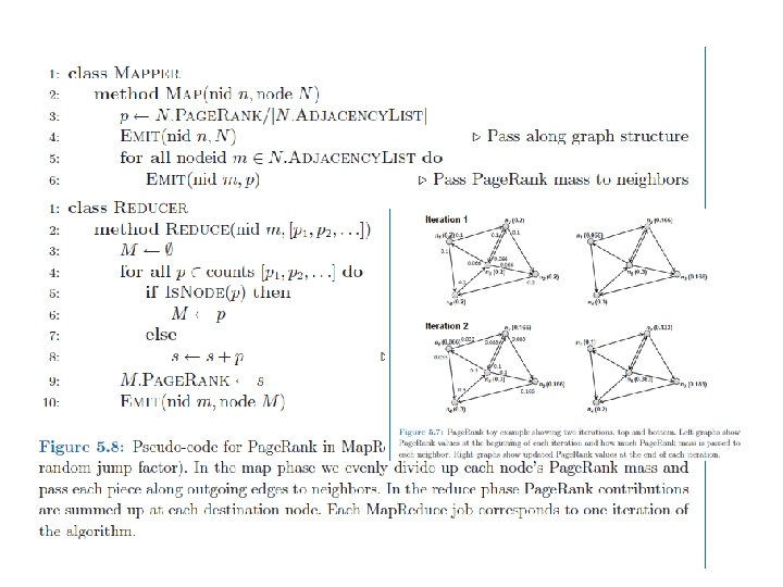
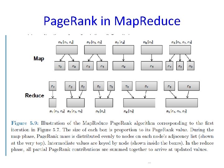
Page. Rank Map. Reduce • Assume alpha=0 • Begins with 5 nodes splitting 1. 0 -> 0. 2 each • Each node must split their 0. 2 to outgoing nodes (map) • Then add up all incoming values (reduce) • Each iteration is one Map. Reduce job

Page. Rank in Map. Reduce Map: distribute Page. Rank “credit” to link targets Reduce: gather up Page. Rank “credit” from multiple sources to compute new Page. Rank value Iterate until convergence . . .

Convergence to end Page Rank • Stop when few changes (some tolerance for precision errors) or reached fixed number of iterations • Driver checks for convergence • How many iterations needed for Page. Rank to converge, e. g. if 322 M edges? – Fewer than expected – 52 iterations

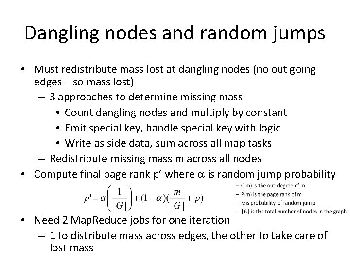
Dangling nodes and random jumps • Must redistribute mass lost at dangling nodes (no out going edges – so mass lost) – 3 approaches to determine missing mass • Count dangling nodes and multiply by constant • Emit special key, handle special key with logic • Write as side data, sum across all map tasks – Redistribute missing mass m across all nodes • Compute final page rank p’ where a is random jump probability • Need 2 Map. Reduce jobs for one iteration – 1 to distribute mass across edges, the other to take care of lost mass

Page. Rank • Assume honest users • No Spider trap – infinite chain of pages all link to single page to inflate Page. Rank • Page. Rank only one of thousands of features used in ranking web pages

Issues with Graph processing • No global data structures can be used • Local computation on each node, results passed to neighbors • With multiple iterations, convergence on global graph • Amount of intermediate data order of number of edges – Worst case? – O(n 2) for dense graph

• CS 591 – read the original Page Rank paper: The anatomy of a large-scale hypertextual Web search engine by S. Brin and L. Page

Issues with Graph processing • Role of combiner?

Page. Rank in Map. Reduce Map: distribute Page. Rank “credit” to link targets Reduce: gather up Page. Rank “credit” from multiple sources to compute new Page. Rank value Iterate until convergence . . .

Dijkstra’s Algorithm Example n 1 n 3 1 10 n 0 0 2 9 3 5 6 7 n 2 Example from CLR 4 n 4 2

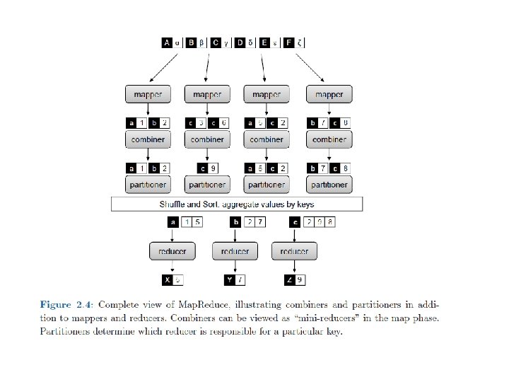
Issues with Graph processing • Combiners only useful if? – can do partial aggregation • Only if multiple nodes being processed by individual mapper and point to same nodes • Otherwise combiner not useful – Assume we have a mapper process more than one node • How to assign nodes (partition graph) so useful?

Issues with Graph processing • Desirable to partition graph so many intracomponent links and few inter-component link • Consider a social network -– Partitioning heuristics – Order nodes by: • • Last name? Zip code? Language spoken? School? – So people are connected

Summary • Graph structure represented with adjacency list • Map over nodes, pass partial results to nodes on adjacency list, partial results aggregated for each node in reducer • Graph structure passed from mapper to reducer, output in same form as input • Algorithms iterative, under control of non. Map. Reduce driver checking for termination at end of each iteration