Learning Parameter Estimation Eran Segal Weizmann Institute Learning

Learning: Parameter Estimation Eran Segal Weizmann Institute

Learning Introduction n So far, we assumed that the networks were given n Where do the networks come from? n n Knowledge engineering with aid of experts Automated construction of networks n Learn by examples or instances

Learning Introduction n Input: dataset of instances D={d[1], . . . d[m]} Output: Bayesian network n Measures of success n n How close is the learned network to the original distribution n n Use distance measures between distributions Often hard because we do not have the true underlying distribution Instead, evaluate performance by how well the network predicts new unseen examples (“test data”) Classification accuracy How close is the structure of the network to the true one? n n n Use distance metric between structures Hard because we do not know the true structure Instead, ask whether independencies learned hold in test data

Prior Knowledge n Prespecified structure n n Prespecified variables n n Learn network structure and CPDs Hidden variables n n Learn only CPDs Learn hidden variables, structure, and CPDs Complete/incomplete data n n Missing data Unobserved variables

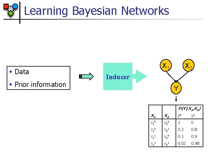
Learning Bayesian Networks § Data § Prior information X 1 X 2 Inducer Y P(Y|X 1, X 2) X 1 X 2 y 0 y 1 x 10 x 20 1 0 x 10 x 21 0. 2 0. 8 x 11 x 20 0. 1 0. 9 x 11 x 21 0. 02 0. 98

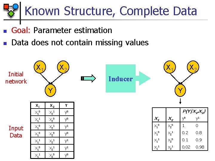
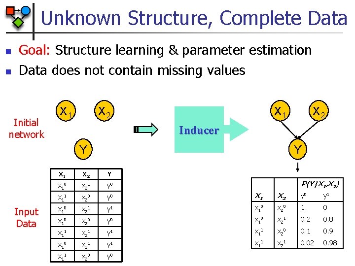
Known Structure, Complete Data n n Goal: Parameter estimation Data does not contain missing values Initial network X 1 X 2 X 1 Inducer Y Input Data X 2 Y X 1 X 2 Y x 10 x 21 y 0 x 11 x 20 y 0 X 1 X 2 y 0 y 1 x 10 x 21 y 1 x 10 x 20 1 0 x 10 x 20 y 0 x 10 x 21 0. 2 0. 8 x 11 x 21 y 1 x 11 x 20 0. 1 0. 9 x 10 x 21 y 1 x 11 x 21 0. 02 0. 98 x 11 x 20 y 0 P(Y|X 1, X 2)

Unknown Structure, Complete Data n n Goal: Structure learning & parameter estimation Data does not contain missing values Initial network X 1 X 2 X 1 Inducer Y Input Data X 2 Y X 1 X 2 Y x 10 x 21 y 0 x 11 x 20 y 0 X 1 X 2 y 0 y 1 x 10 x 21 y 1 x 10 x 20 1 0 x 10 x 20 y 0 x 10 x 21 0. 2 0. 8 x 11 x 21 y 1 x 11 x 20 0. 1 0. 9 x 10 x 21 y 1 x 11 x 21 0. 02 0. 98 x 11 x 20 y 0 P(Y|X 1, X 2)

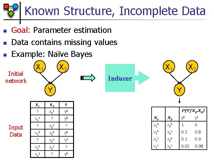
Known Structure, Incomplete Data n n n Goal: Parameter estimation Data contains missing values Example: Naïve Bayes Initial network X 1 X 2 X 1 Inducer Y Input Data X 2 Y X 1 X 2 Y ? x 21 y 0 x 11 ? y 0 X 1 X 2 y 0 y 1 ? x 21 ? x 10 x 20 1 0 x 10 x 20 y 0 x 10 x 21 0. 2 0. 8 ? x 21 y 1 x 11 x 20 0. 1 0. 9 x 10 x 21 ? x 11 x 21 0. 02 0. 98 x 11 ? y 0 P(Y|X 1, X 2)

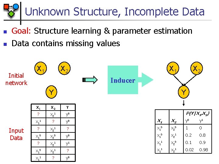
Unknown Structure, Incomplete Data n n Goal: Structure learning & parameter estimation Data contains missing values Initial network X 1 X 2 X 1 Inducer Y Input Data X 2 Y X 1 X 2 Y ? x 21 y 0 x 11 ? y 0 X 1 X 2 y 0 y 1 ? x 21 ? x 10 x 20 1 0 x 10 x 20 y 0 x 10 x 21 0. 2 0. 8 ? x 21 y 1 x 11 x 20 0. 1 0. 9 x 10 x 21 ? x 11 x 21 0. 02 0. 98 x 11 ? y 0 P(Y|X 1, X 2)

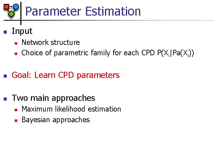
Parameter Estimation n Input n n Network structure Choice of parametric family for each CPD P(Xi|Pa(Xi)) n Goal: Learn CPD parameters n Two main approaches n n Maximum likelihood estimation Bayesian approaches

Biased Coin Toss Example n Coin can land in two positions: Head or Tail n Estimation task n n Given toss examples x[1], . . . x[m] estimate P(H)= and P(T)= 1 - Assumption: i. i. d samples n n n Tosses are controlled by an (unknown) parameter Tosses are sampled from the same distribution Tosses are independent of each other

Biased Coin Toss Example Goal: find [0, 1] that predicts the data well n “Predicts the data well” = likelihood of the data given n Example: probability of sequence H, T, T, H, H L(D: ) n 0 0. 2 0. 4 0. 6 0. 8 1

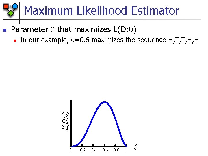
Maximum Likelihood Estimator Parameter that maximizes L(D: ) n In our example, =0. 6 maximizes the sequence H, T, T, H, H L(D: ) n 0 0. 2 0. 4 0. 6 0. 8 1

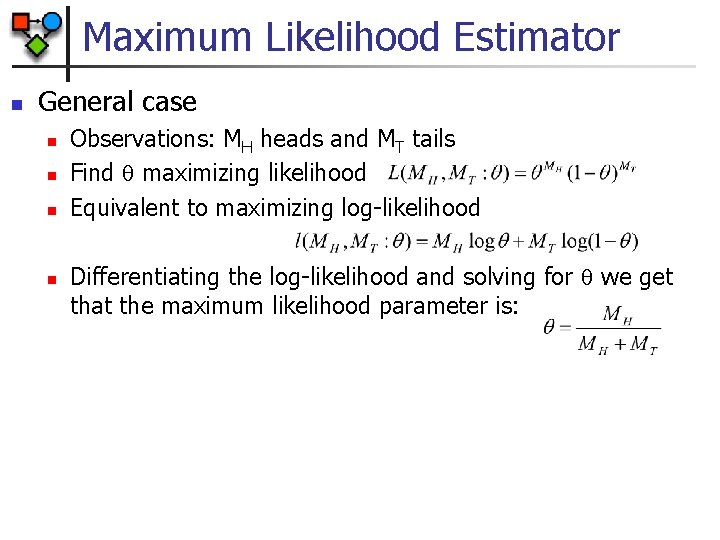
Maximum Likelihood Estimator n General case n n Observations: MH heads and MT tails Find maximizing likelihood Equivalent to maximizing log-likelihood Differentiating the log-likelihood and solving for we get that the maximum likelihood parameter is:

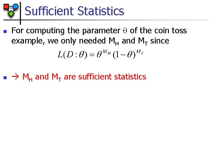
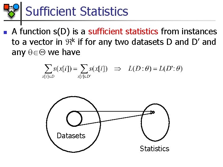
Sufficient Statistics n n For computing the parameter of the coin toss example, we only needed MH and MT since MH and MT are sufficient statistics

Sufficient Statistics n A function s(D) is a sufficient statistics from instances to a vector in k if for any two datasets D and D’ and any we have Datasets Statistics

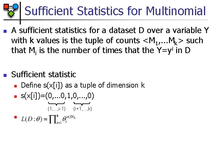
Sufficient Statistics for Multinomial n n A sufficient statistics for a dataset D over a variable Y with k values is the tuple of counts <M 1, . . . Mk> such that Mi is the number of times that the Y=yi in D Sufficient statistic n n Define s(x[i]) as a tuple of dimension k s(x[i])=(0, . . . 0, 1, 0, . . . , 0) (1, . . . , i-1) n (i+1, . . . , k)

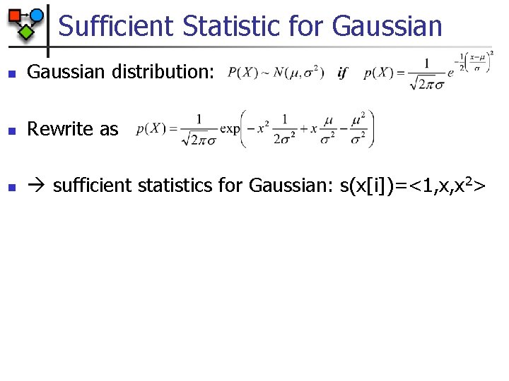
Sufficient Statistic for Gaussian n Gaussian distribution: n Rewrite as n sufficient statistics for Gaussian: s(x[i])=<1, x, x 2>

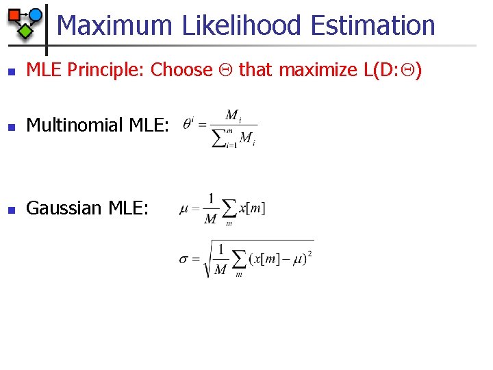
Maximum Likelihood Estimation n MLE Principle: Choose that maximize L(D: ) n Multinomial MLE: n Gaussian MLE:

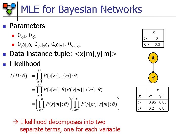
MLE for Bayesian Networks n Parameters n n X x 0 , x 1 y 0|x 0, y 1|x 0, y 0|x 1, y 1|x 1 Data instance tuple: <x[m], y[m]> Likelihood x 0 x 1 0. 7 0. 3 X Y Y Likelihood decomposes into two separate terms, one for each variable X y 0 y 1 x 0 0. 95 0. 05 x 1 0. 2 0. 8

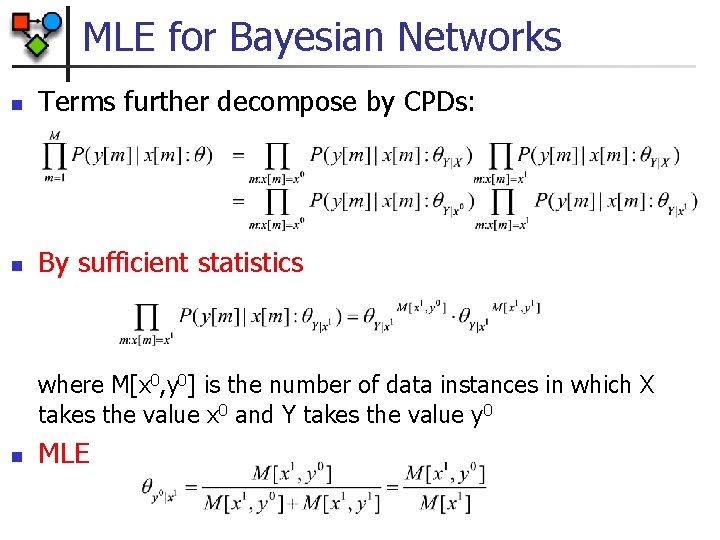
MLE for Bayesian Networks n Terms further decompose by CPDs: n By sufficient statistics where M[x 0, y 0] is the number of data instances in which X takes the value x 0 and Y takes the value y 0 n MLE

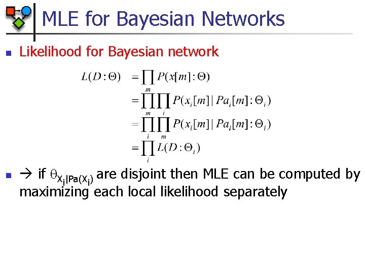
MLE for Bayesian Networks n n Likelihood for Bayesian network if Xi|Pa(Xi) are disjoint then MLE can be computed by maximizing each local likelihood separately

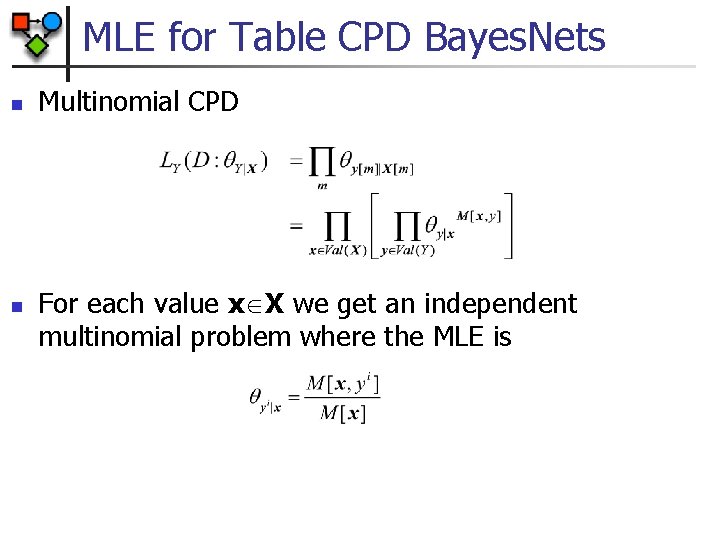
MLE for Table CPD Bayes. Nets n n Multinomial CPD For each value x X we get an independent multinomial problem where the MLE is

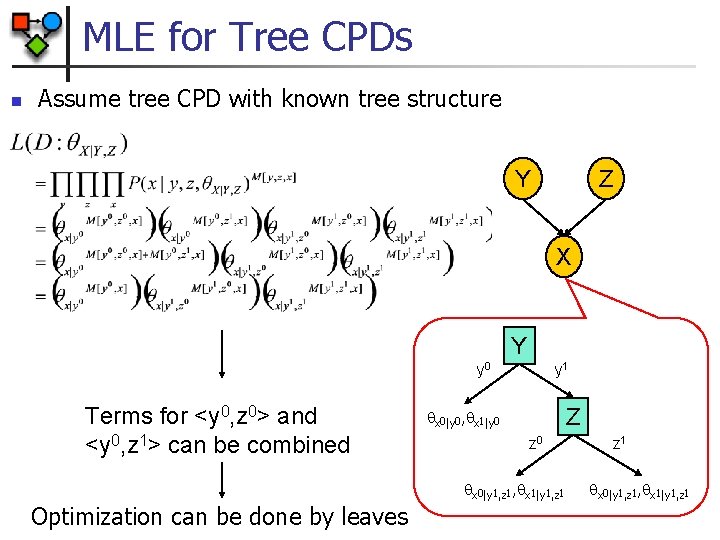
MLE for Tree CPDs n Assume tree CPD with known tree structure Y Z X Y y 0 Terms for <y 0, z 0> and <y 0, z 1> can be combined y 1 Z x 0|y 0, x 1|y 0 z 0 x 0|y 1, z 1, x 1|y 1, z 1 Optimization can be done by leaves z 1 x 0|y 1, z 1, x 1|y 1, z 1

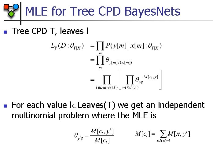
MLE for Tree CPD Bayes. Nets n n Tree CPD T, leaves l For each value l Leaves(T) we get an independent multinomial problem where the MLE is

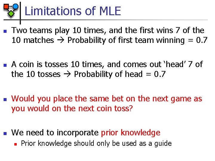
Limitations of MLE n n Two teams play 10 times, and the first wins 7 of the 10 matches Probability of first team winning = 0. 7 A coin is tosses 10 times, and comes out ‘head’ 7 of the 10 tosses Probability of head = 0. 7 Would you place the same bet on the next game as you would on the next coin toss? We need to incorporate prior knowledge n Prior knowledge should only be used as a guide

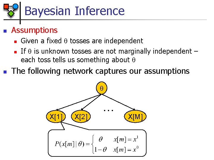
Bayesian Inference n Assumptions n n n Given a fixed tosses are independent If is unknown tosses are not marginally independent – each toss tells us something about The following network captures our assumptions X[1] X[2] … X[M]

Bayesian Inference n Joint probabilistic model X[1] n X[2] … X[M] Posterior probability over Likelihood Prior For a uniform prior, posterior is the normalized likelihood Normalizing factor

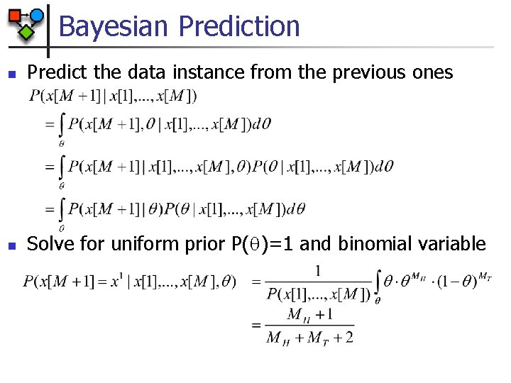
Bayesian Prediction n Predict the data instance from the previous ones n Solve for uniform prior P( )=1 and binomial variable

Example: Binomial Data n Prior: uniform for in [0, 1] n n P( ) = 1 P( |D) is proportional to the likelihood L(D: ) (MH, MT ) = (4, 1) n n MLE for P(X=H) is 4/5 = 0. 8 Bayesian prediction is 5/7 0 0. 2 0. 4 0. 6 0. 8 1

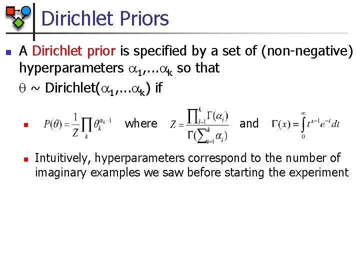
Dirichlet Priors n A Dirichlet prior is specified by a set of (non-negative) hyperparameters 1, . . . k so that ~ Dirichlet( 1, . . . k) if n n where and Intuitively, hyperparameters correspond to the number of imaginary examples we saw before starting the experiment

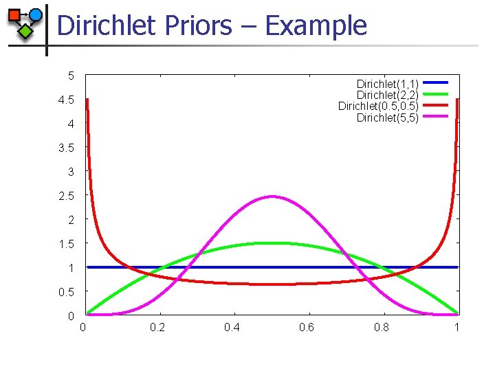
Dirichlet Priors – Example 5 Dirichlet(1, 1) Dirichlet(2, 2) Dirichlet(0. 5, 0. 5) Dirichlet(5, 5) 4. 5 4 3. 5 3 2. 5 2 1. 5 1 0. 5 0 0 0. 2 0. 4 0. 6 0. 8 1

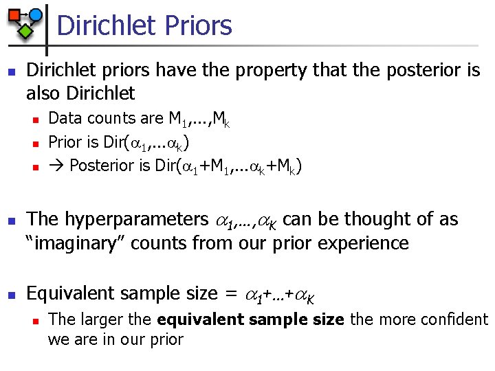
Dirichlet Priors n Dirichlet priors have the property that the posterior is also Dirichlet n n n Data counts are M 1, . . . , Mk Prior is Dir( 1, . . . k) Posterior is Dir( 1+M 1, . . . k+Mk) The hyperparameters 1, …, K can be thought of as “imaginary” counts from our prior experience Equivalent sample size = 1+…+ K n The larger the equivalent sample size the more confident we are in our prior

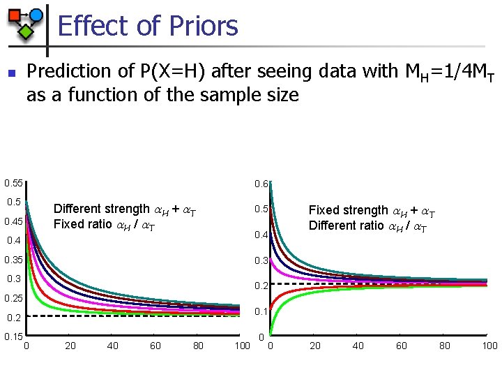
Effect of Priors n Prediction of P(X=H) after seeing data with MH=1/4 MT as a function of the sample size 0. 55 0. 6 0. 5 Different strength H + T Fixed ratio H / T 0. 45 0. 4 0. 35 Fixed strength H + T Different ratio H / T 0. 3 0. 25 0. 1 0. 2 0. 15 0 20 40 60 80 100 0 0 20 40 60 80 100

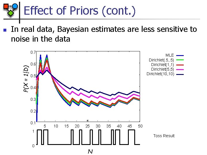
Effect of Priors (cont. ) In real data, Bayesian estimates are less sensitive to noise in the data 0. 7 P(X = 1|D) n MLE Dirichlet(. 5, . 5) Dirichlet(1, 1) Dirichlet(5, 5) Dirichlet(10, 10) 0. 6 0. 5 0. 4 0. 3 0. 2 0. 1 N 5 10 15 20 25 30 35 40 45 50 1 Toss Result 0 N

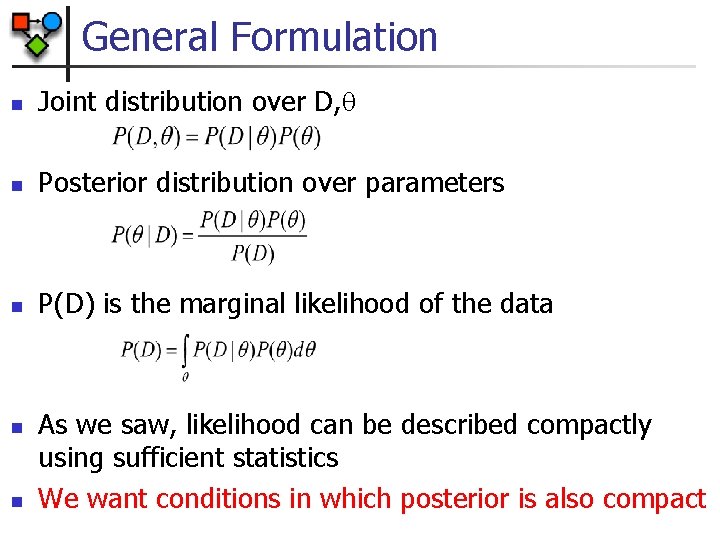
General Formulation n Joint distribution over D, n Posterior distribution over parameters n P(D) is the marginal likelihood of the data n n As we saw, likelihood can be described compactly using sufficient statistics We want conditions in which posterior is also compact

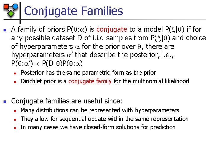
Conjugate Families n A family of priors P( : ) is conjugate to a model P( | ) if for any possible dataset D of i. i. d samples from P( | ) and choice of hyperparameters for the prior over , there are hyperparameters ’ that describe the posterior, i. e. , P( : ’) P(D| )P( : ) n n n Posterior has the same parametric form as the prior Dirichlet prior is a conjugate family for the multinomial likelihood Conjugate families are useful since: n n n Many distributions can be represented with hyperparameters They allow for sequential update within the same representation In many cases we have closed-form solutions for prediction

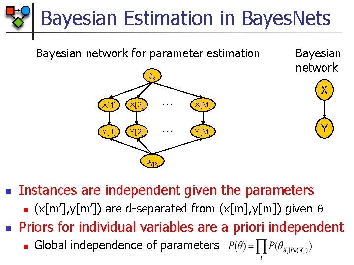
Bayesian Estimation in Bayes. Nets Bayesian network for parameter estimation X Bayesian network X X[1] X[2] … X[M] Y[1] Y[2] … Y[M] Y Y|X n Instances are independent given the parameters n n (x[m’], y[m’]) are d-separated from (x[m], y[m]) given Priors for individual variables are a priori independent n Global independence of parameters

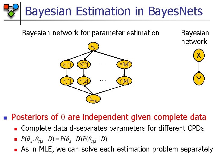
Bayesian Estimation in Bayes. Nets Bayesian network for parameter estimation X Bayesian network X X[1] X[2] … X[M] Y[1] Y[2] … Y[M] Y Y|X n Posteriors of are independent given complete data n Complete data d-separates parameters for different CPDs n n As in MLE, we can solve each estimation problem separately

Bayesian Estimation in Bayes. Nets Bayesian network for parameter estimation X X[1] X[2] … X[M] Y[1] Y[2] … Y[M] Y|X=0 Bayesian network Y Y|X=1 Posteriors of are independent given complete data n n Also holds for parameters within families Note context specific independence between Y|X=0 and Y|X=1 when given both X and Y

Bayesian Estimation in Bayes. Nets Bayesian network for parameter estimation X X[1] X[2] … X[M] Y[1] Y[2] … Y[M] Y|X=0 Bayesian network Y Y|X=1 Posteriors of can be computed independently n n For multinomial Xi|pai posterior is Dirichlet with parameters Xi=1|pai+M[Xi=1|pai], . . . , Xi=k|pai+M[Xi=k|pai]

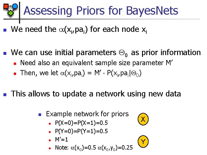
Assessing Priors for Bayes. Nets n We need the (xi, pai) for each node xi n We can use initial parameters 0 as prior information n Need also an equivalent sample size parameter M’ Then, we let (xi, pai) = M’ P(xi, pai| 0) This allows to update a network using new data n Example network for priors n n P(X=0)=P(X=1)=0. 5 P(Y=0)=P(Y=1)=0. 5 M’=1 Note: (x 0)=0. 5 (x 0, y 0)=0. 25 X Y

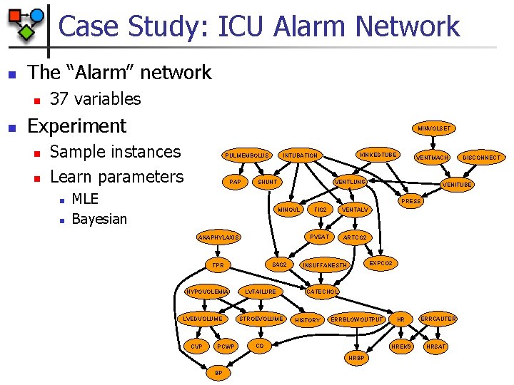
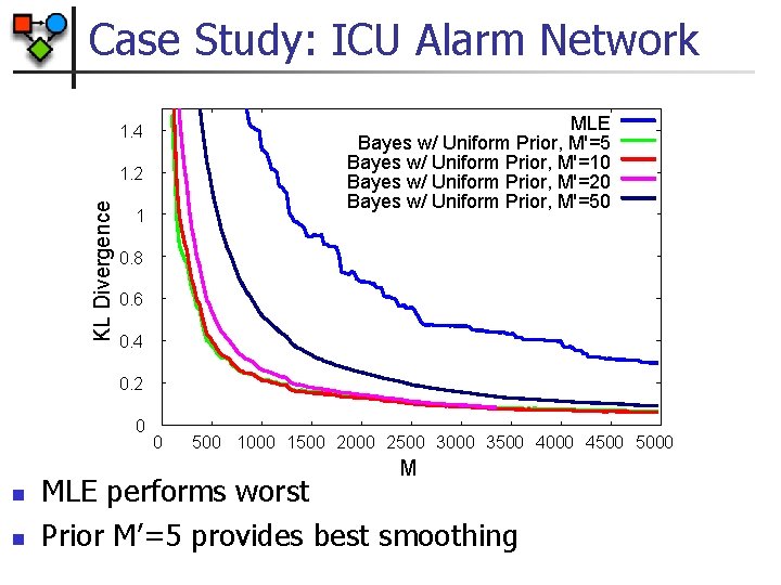
Case Study: ICU Alarm Network n The “Alarm” network n n 37 variables Experiment n n MINVOLSET Sample instances Learn parameters n n PULMEMBOLUS PAP KINKEDTUBE INTUBATION SHUNT MLE Bayesian VENTMACH VENTLUNG VENITUBE PRESS MINOVL ANAPHYLAXIS SAO 2 TPR HYPOVOLEMIA LVEDVOLUME CVP PCWP LVFAILURE STROEVOLUME FIO 2 VENTALV PVSAT ARTCO 2 EXPCO 2 INSUFFANESTH CATECHOL HISTORY ERRBLOWOUTPUT CO BP HR HREKG HRBP DISCONNECT ERRCAUTER HRSAT

Case Study: ICU Alarm Network MLE Bayes w/ Uniform Prior, M'=5 Bayes w/ Uniform Prior, M'=10 Bayes w/ Uniform Prior, M'=20 Bayes w/ Uniform Prior, M'=50 1. 4 KL Divergence 1. 2 1 0. 8 0. 6 0. 4 0. 2 0 0 500 1000 1500 2000 2500 3000 3500 4000 4500 5000 M n n MLE performs worst Prior M’=5 provides best smoothing

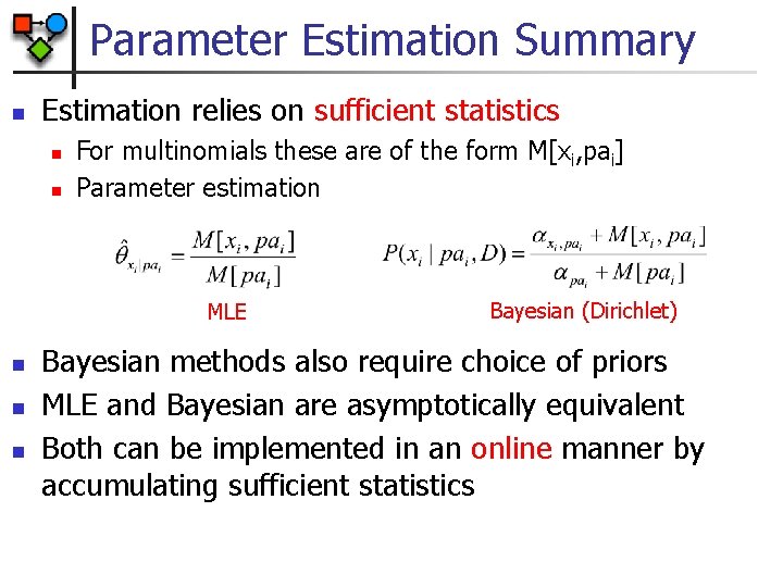
Parameter Estimation Summary n Estimation relies on sufficient statistics n n For multinomials these are of the form M[xi, pai] Parameter estimation MLE n n n Bayesian (Dirichlet) Bayesian methods also require choice of priors MLE and Bayesian are asymptotically equivalent Both can be implemented in an online manner by accumulating sufficient statistics