Karakteristini morfometrijski parametri znaajni za definisanje geometrijskogmatematikog modela

Karakteristični morfometrijski parametri značajni za definisanje geometrijskog/matematičkog modela BUTNE KOSTI Doc. dr Stojanka Arsić 4. Sastanak projektnog tima 29. 11. 2008 Mašinski fakultet Niš

FEMUR / PROKSIMALNI OKRAJAK Karakteristični morfometrijski parametri značajni za definisanje geometrijskog/matematičkog modela Doc. dr Stojanka Arsić 4. Sastanak projektnog tima 29. 11. 2008 Mašinski fakultet Niš

FEMUR- butna kost DELOVI 1. GORNJI OKRAJAK (extremitas proximalis) 2. TELO ( corpus femoris) 3. DONJI OKRAJAK ( ekstremitas distalis)

FEMUR- butna kost GORNJI OKRAJAK (extremitas proximalis)

ZGLOBNE POVRŠINE NA GORNJEM I DONJEM OKRAJKUFEMURA

ZGLOBNE POVRŠINE NA GORNJEM OKRAJKUFEMURA

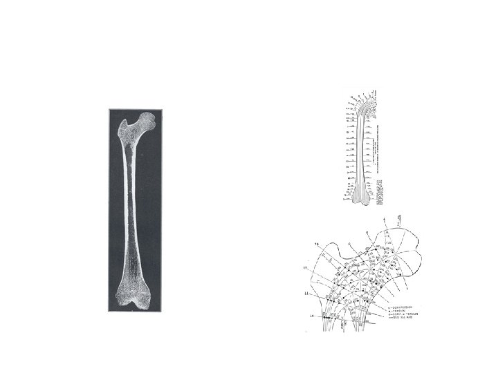
DA SILVA, V. J. ; ODA, J. Y. & SANT'ANA, D. M. G. Anatomical aspects of the proximal femur of adults brazilians. Int. J. Morphol. , 21(4): 303 308, 2003. The following morphometric measures were made: angle of the femur neck, 1. angle of the femur neck, 2. circumference of the femur head and neck, 3. length of the femur neck and 4. length of the whole bone. The comparative analysis of the 5. angle of the femur neck between the right and left sides

The comparative analysis of the 5. angle of the femur neck between the right and left sides of adults demonstrated values similar to those described in the classic literature for adults with mean significantly smaller on the right side (122. 5 o) than on the left side (125. 6 o). As for the length of the femur neck in this study larger values on the left side (23. 5 mm) than on the right side (22. 3 mm) were observed

Angle of the femur neck (ACF): angle between the neck and the diaphysis, using a goniometer Fig. 1. Schematic representation of the proximal epiphysis of the femur demonstrating the reference points for the morphometry of the angle of the femur neck (ACF)

• Length of the femur (CF): a line was drawn along the bone from the median point of the proximal epiphysis to that of the distal epiphysis. • Length of the femur neck (CCF): straight line distance from the base of the greater trochanter to the inferior region of the head (Fig. 2).

. Fig 2. Schematic representation of the proximal epiphysis of the femur demonstrating the reference points for the morphometry. CCF length of the femur neck.

Circumference of the median points of the femur neck and head Fig. 3. Schematic representation of the proximal epiphysis of the femur demonstrating the reference points for the morphometry. Cca. F circumference of the femur head.

The articular trochanteric distance

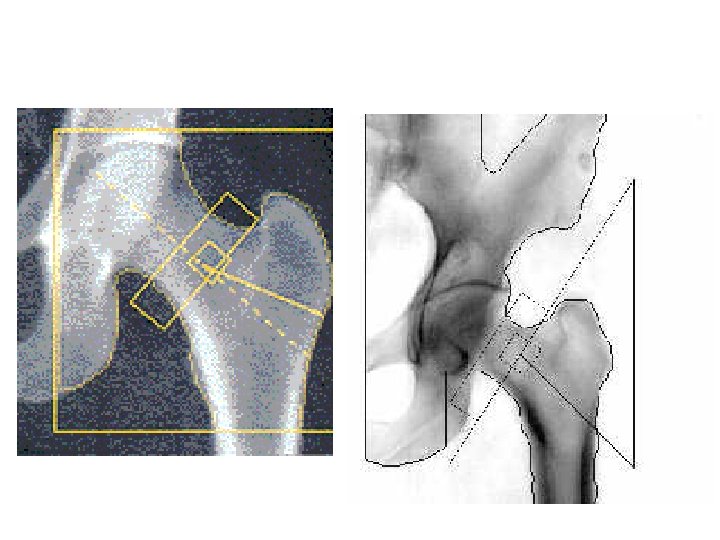
Parameters commonly used to evaluate proximal femur geometry. A, Neck shaft angle; B, Femoral neck axis length or femoral neck length; Taken from: Bouxsein M, Karasik D: Bone Geometry and Skeletal Fragility. Current Osteoporosis Reports. 4(2): 49 56. Current Medicine Group LLC.

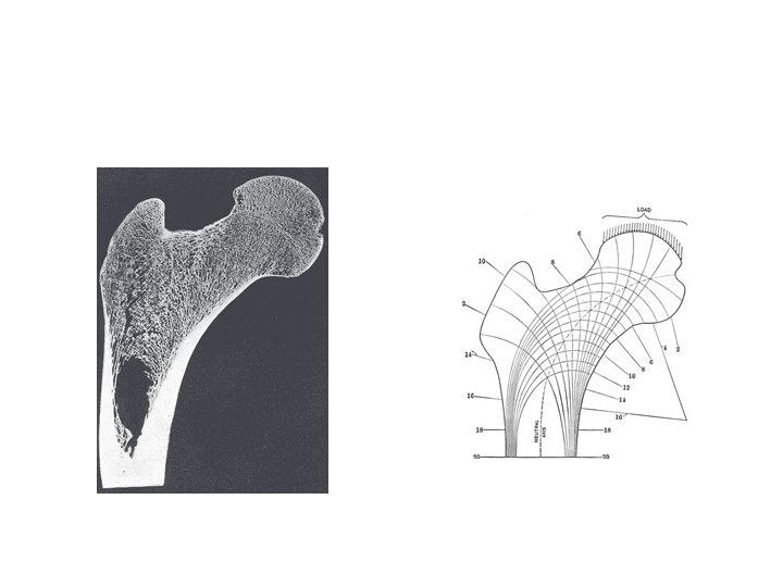
The human hip joint. Radiograph of the human proximal femur and acetabulum in which the two main systems of trabeculae (group 1 and 2) are indicated. These are traditionally known as the principle tensile and compressive trabeculae respectively, a questionable nomenclature. Rudman et al. Bio. Medical Engineering On. Line 2006 5: 12 doi: 10. 1186/1475 925 X 5 12

• Compression or tension? The stress distribution in the proximal femur • KE Rudman , RM Aspden and JR Meakin Department of Orthopaedic Surgery, University of Aberdeen, Foresterhill, Aberdeen, AB 25 2 ZD, UK • Bio. Medical Engineering On. Line 2006, 5: 12 doi: 10. 1186/1475 925 X 5 12

• Mechanically Mediated Bone Adaptation bone mechanical properties depend significantly on bone tissue structure Mechanically Mediated Bone Adaptation Theories (1865 1920) Theories of how mechanical stimulus affected bone adaptation begin in earnest about the time the American Civil War was ending. In 1867, a German anatomist Von Meyer received a grant from the Prussian government to study skeletal posture. As part of this grant, Von Meyer studied trabecular orientation in the proximal femur. While presenting these results at a scientific meeting, a Swiss engineer named Culmann noticed that Von Meyer's trabecular drawings bore a striking resemblance to principal stress lines Culmann had determined for a crane.

The trabecular drawings and crane principal stress lines

– Diagram of the lines of stress in the upper femur, based upon the mathematical analysis of the right femur. These result from the combination of the different kinds of stresses at each point in the femur. (After Koch. )

– Intensity of the maximum tensile and compressive stresses in the upper femur. Computed for the load of 100 pounds on the right femur. Corresponds to the upper part of the previous figure. (After Koch. )

Diagram of the computed lines of maximum stress in the normal femur. The section numbers 2, 4, 6, 8, etc. , show the positions of the transverse sections analyzed. The amounts of the maximum tensile and compressive stress at the various sections are given for a load of 100 pounds on the femur head. For the standing position (“at attention”) these stresses are multiplied by 0. 6, for walking by 1. 6 and for running by 3. 2. (After Koch. )

FIG. 249– Frontal longitudinal midsection of left femur. Taken from the same subject as the one that was analyzed and shown in Figs. 248 and 250. 4/9 of natural size. (After Koch. )

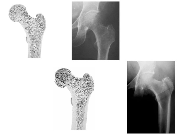
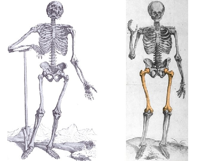
Forces as much as 6 x body weight are transmitted across the hip. The bone remodels according to the forces applied (Wolff's law) and this is reflected in the trabecular pattern illustrated above. This is highly relevant to fracture mechanism and fixation.

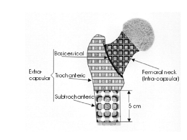
The image shows the regions usually measured on the proximal femur: NECK, TROCHANTERIC, AND INTER-TROCHANTERIC. All three together form the "total hip" which is not actually the hip joint at all. Ignore "Ward's triangle" which is an unreliable square. Note that the trochanteric region is less dense because it has more trabecular bone. Also, it is critically important that the cutoff line at the bottom is in the standard place, because even one pixel will include more of the dense bone of the shaft and make the measurement inaccurate.

This is an image from Lunar. The newer densitometers include the total hip, the older ones only the neck and trochanter.

Recommendations for BMD Testing BMD of the hip can be measured at several regions, including the femoral neck, trochanteric, intertrochanteric, Ward's Triangle and/or total hip. With the large region of interest in the total hip, measurement errors may be minimized. However, caution must be used in measuring Ward's triangle; its small area introduces a higher possibility of measurement error and the anatomic site itself may be variably defined by different manufacturers. 27 Unlike the spine, where cancellous bone is uniformly distributed and, thus, shows a uniform pattern of bone loss, the hip shows variable BMD because different areas of the femur are composed of different percentages of cancellous bone, and have different risks of fracture. 28

Result a virtual load testing a femur by using a CT based Finite Element Method. (Fig. 1) The result of the stance configuration (left). The predicted fracture line (red line) located at the femoral neck. The result of the fall configuration (right). The predicted fracture line appeared at the femoral trochanteric region. The color bar represents maximum principal stress.

• The Department of Orthopaedic Surgery, The University of Tokyo. Graduate School of Information Science and Technology, The University of Tokyo. • Objects • To develop a non invasive method for predicting bone strength. • To develop osteosynthetic devices. • Major Research Projects Orthopedic biomechanics Bone mechanics Mechanobiology External fixation biomechanics Basic research for metallic materials for osteosynthesis

• Identification of hip fracture patients from radiographs using Fourier analysis of the trabecular structure: a cross-sectional study • Jennifer S Gregory 1 , Alison Stewart 2 , Peter E Undrill 3 , David M Reid 2 and Richard M Aspden 1

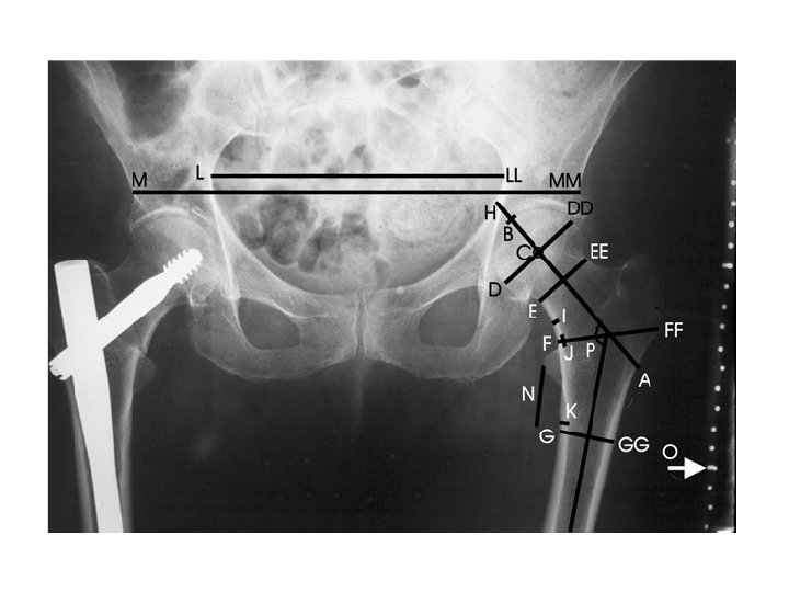
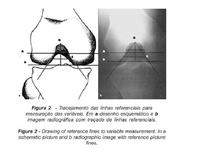
Regions of interest. Displays the five regions of interest, upper femoral head (UH), central femoral head (CH), upper femoral neck (UN), Ward's triangle area (WA) and the lower femoral neck (LN) used for analysis. Points A to G are determined by the femoral head and neck and used to locate the ROIs. Points A and E mark the femoral neck width. Points B, C and D lie at 1/4, 1/2 and 3/4 along this line. Point F is the centre point of the femoral head, point G at 1/2 the radius of the femoral head at an angle of 45 degrees to the neck width, 135 degrees to the neck shaft, shown as a dashed line through point C. Gregory et al. BMC Medical Imaging 2004 4: 4

• • • Profile generation. (A) Shows a typical region of interest (contrast enhanced for visualisation) showing the trabecular bone structure, in this case aligned approximately 22° to the vertical. (B) The central section of the FFT (128 × 128 pixels). The horizontal and vertical axes have been marked with a mid grey tone to indicate that they have been excluded from the angle calculation. The bright strip at the centre (running from top left to bottom right) shows the preferred orientation of the trabeculae. Angles calculated from the Fourier power spectrum correspond to the same angles in the spatial domain, rotated by 90°. (C) The pixels with the maximum values are marked using white squares for the first 25 spatial frequency values of the Fourier power spectrum. The median angle, lying 21. 8° from the horizontal is shown by a dashed white line. (D)_The regions used to generate the parallel (shaded black) and perpendicular (shaded white) profiles, based on the orientation of the trabecular structure. Gregory et al. BMC Medical Imaging 2004 4: 4 doi: 10. 1186/1471 2342 4 4 Download authors' original image

Hip Axis Length HAL • single best predictor of hip fracture is femoral bone density. But bone density is not the only factor influencing weather or not a fracture will occur. • According to engineering principals, strength depends on • (1) the mechanical properties of the materials, • (2) the objects geometry and shape, and, • (3) the loading conditions, in terms of magnitude, rate, and direction, of force applied to the object. • If geometry of the hip is related to fracture risk, geometric measurements might be used together with densitometric evaluations for a better assessment of hip fracture risk than might be obtained from just a density measurement alone. • Prospective studies show that HAL has demonstrated the ability to predict fractures!1 1. Faulkner K. , Advanced Hip Assessment, GE Medical Systems Lunar, July 2001

Key Measurements Each centimeter (10%) increase in Hip Axis length (HAL) increases hip fracture by 50 80% depending on the study. For short term prediction of hip fracture (within 2 years), HAL was shown to predict hip fractures independent of BMD. 1 1. Faulkner K. , Advanced Hip Assessment, GE Medical Systems Lunar, July 2001

Dual. Femur With the Dual. Femur option, both femora are automatically scanned in one seamless acquisition without repositioning the patient. As such Dual. Femur allows you to assess the density of the critical hip region, including identification of the weakest side increasing confidence in your treatment decisions. In addition, the trending function enables seamless follow up of change over time.

• The Dual. Femur application atomically measures, and averages, both the left and right femora in one measurement sequence. • This procedure promises to improve diagnostic accuracy by identifying the femur with the lowest density. An equally important benefit is a 30% decrease in precision error, which improves sensitivity for monitoring response at the femur itself! • . Faulkner K. , Advanced Hip Assessment, GE Medical Systems Lunar, July 2001

Upper Neck Region The Upper Neck Region is comprised of the upper half of the standard Neck region. This new region is highly sensitive to bone loss and is can be used as an early predictor of trochanteric and neck fractures. 1 1. Faulkner K. , Advanced Hip Assessment, GE Medical Systems Lunar, July 2001

• The upper portion of the femoral neck has been reported to be a sensitive predictor of neck fractures. Studies have demonstrated that femoral fractures are usually initiated in the upper neck region. The thickness and porosity of the bone in the upper neck region is believed to be critical to maintaining femoral strength. The upper neck demonstrates a more rapid age related decline than the standard femoral neck region, suggesting it may provide some advantage for early detection of osteoporosis. 1 1. Faulkner K. , Advanced Hip Assessment, GE Medical Systems Lunar, July 2001

The femoral neck torsion angle (FNTA) is the angle between the axis of the femoral neck (cervical plane) and the coronal plane of the femoral condyles (condylar plane). If the neck is oriented forward with respect to the condylar plane, it is referred to as anteversion (positive FNTA).

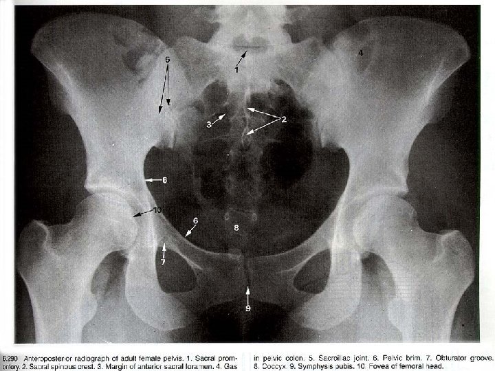
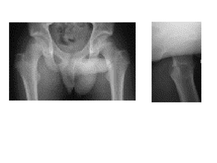
Radiograph of the hip region: Identify the following on a radiograph of the hip region: • ilium • ischium • pubis • pubic symphysis • sacroiliac joint • acetabular lip • head of femur • neck of femur • greater trochanter • lesser trochanter

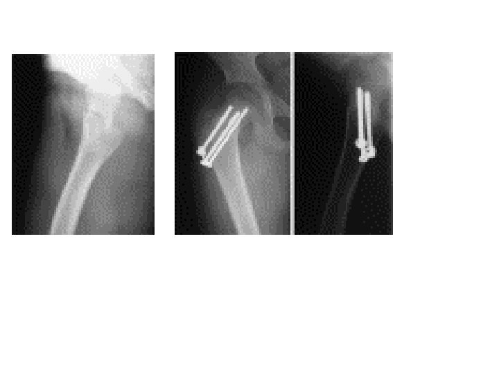
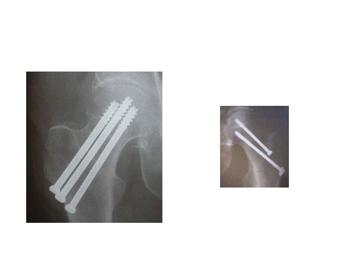
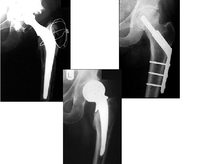
The Functional Fit • The ITST Intramedullary Nail System is designed to treat unstable, comminuted, proximal fractures of the femur, specifically, the intertrochanteric and subtrochanteric regions. The ITST design is truly versatile in offering the combined features of intramedullary nail and hip screw systems.

True Anatomic Design Proximal design features an anatomic 5° Lateral Bend, which allows for the less invasive trochanteric starting point to be utilized. Inserted into the femoral head at 130°, the most common angle used in gliding nails. 15° anteversion of the proximal holes for easier passage of the nail down the femoral canal, and simpler distal freehand targeting. Range of distal diameters accommodates anatomic fit.

Natural Proximal Geometry • Construct is a high strength stainless steel alloy, 22 13 5, which allows the implant more design freedom, while maintaining adequate implant strength. • Proximal geometry features a bone conserving diameter of 16. 5 mm. • Accommodates an 11 mm Lag Screw, providing a high level of proximal bone implant interface. • The height of the proximal nail diameter combined with a short transition region allows for easy insertion of the Lag Screw across the femoral neck, without the concern of the nail sitting too proud or too deep in the bone. • True Anatomic Design

Implant geometry

Implant geometry Caracterisation of the risk of dislocation of a prosthetic configuration by the distance AB Dislocation occurs when the head moves from point A to point B The risk diminished when AB increases AB is determined by, size of the head, depth of the cup, degree of incline AB characterises a system in terms of risk of dislocation AB = R head x √ 2 x (1 – cosα ) By Massé and Wagner

Implant geometry • When we look at the external geometry of the today’s implant, it is a press fit hemisphere which is extended in the equatorial region cylindrically by 3 mm (figure 7). The pole is slightly flattened by removing 0. 5 mm of metal in order to optimise impaction and enhance the press fit. The equatorial press fit is augmented by an even band of slightly raised ridges which ensure primary stability. These ridges form a very even macrostructure around the equatorial rim, but the geometry is in keeping with Gilles Bousquets three point fixation concept. The press fit is optimised at the levels of the ilium, ischium and pubis due to the macrostructure rides being more raised at these points (figure 7).

Figure 7: Primary fixation mode of the NOVAE cups External geometry 1/2 sphere +3 mm equator Pole flattened by 0. 5 mm + Zone of equatorial press fit Details of concept

• If the cup comes across as being cylindro – spherical, its geometry is more complex. It is in fact a cup with a raised superior portion. • The geometry of todays cup in effect comes from the original geometry which was chamfered in the lower (inferior) zone and extended in the upper (superior) zone, which resulted in an 8 mm cap extending from the equator of the hemisphere

Figure 8: Evolution of the geometry of the cup 1/2 sphere Cap Section through cylinder and ½ sphere Novae 1: previous generation Superior point Inferior point Elimination of lateral edges (protuberances) Novae 1 => Novae Evolution

Fig 3: Measurement of diameter of femoral head

Method of measurement of diameter of acetabulam

Fig 1: Method of measurement of depth of acetabulam

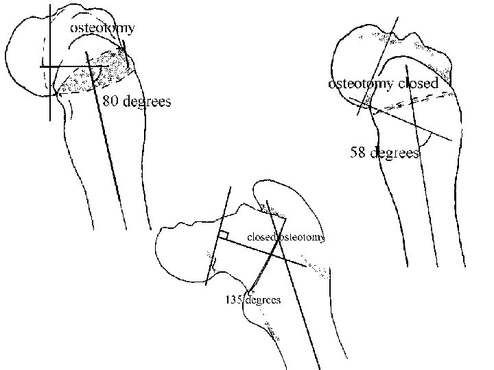
Osteotomy

Deformable Lower Extremity Model • graphics based model of the human lower extremity with a "deformable" femur. • This model characterizes the geometry of the pelvis, femur, and proximal tibia, the kinematics of the hip and tibiofemoral joints, and the paths of the medial hamstrings, iliopsoas, and adductor muscles for an average sized adult male. • The femur of our deformable model can be altered to represent anteversion angles of 0 60°, neck shaft angles of 110 150°, and/or neck lengths of 35 60 mm. The lesser trochanter torsion angle of the model can be adjusted by as much as 30° anteriorly or 10° posteriorly. Hence, this model enables rapid and accurate estimation of muscle tendon lengths and moment arms for individuals with a wide range of movement abnormalities and femoral deformities.

"deformable" femur. Deformable model in action. We can deform the femur of our generic model (left, shaded bone) to resemble the deformed femurs of children with cerebral palsy (wireframe bone) by increasing its femoral anteversion angle (middle) and its neckshaft angle (right).

• Associated Publications • Arnold and Delp. Rotational moment arms of the hamstrings and adductors vary with femoral geometry and limb position: implications for the treatment of internally rotated gait. Journal of Biomechanics, 2001. (Download PDF) • Arnold, Blemker, and Delp. Evaluation of a deformable musculoskeletal model for estimating muscle tendon lengths during crouch gait. Annals of Biomedical Engineeering, 2001. (Download PDF)

• A new value of proximal femur geometry to evaluate hip fracture risk: true moment arm. • Ulusoy H, Bilgici A, Kuru O, Sarica N, Arslan S, Erkorkmaz U. • Hip Int. 2008 Apr-Jun; 18(2): 101 -7. • This study was undertaken to determine the influence of proximal femur geometry on hip fracture risk independent of bone mineral density

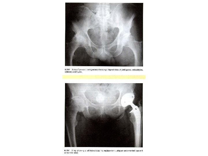
Glinkowski Wojciech; Ciszek Bogdan Antomy of the Proximal Femur -geometry and architecture. Morphologic investigation and literature review. Ortopedia, traumatologia, rehabilitacja 2002; 4(2): 200 8 • Material and methods. To analyze morphology and endosteal anatomy of the proximal ends of the femur of 40 cadaver femora were x rayed, dissected and measured. Various variables including trabecular pattern, calcar size, and cortical bone were measured and correlated. Observations were compared to literature concerns the various aspects of anatomy of the proximal femur. <br /> Results. One must recognize that much of the information that we gather in every day practice is two dimensional, namely, x rays of the hip. Morphological data with three dimensional perspective demonstrate internal architecture of proximal femur including calcar femorale. Authors pointed out lower values of neck shaft angle than observed in other examined populations. <br /> Conclusions. They found that topographic and angular position of calcar femorale depends on anteversion angle. Shadow of the calcar on X ray of the femur in Lauenstein's view may become invisible in some cases what is correlated to its real dimension. Calcar femorale as a anatomical structure has no strict topographic coincidence with "calcar resorption" observed in some total hip replacements.

Differences in proximal femur geometry distinguish vertebral from femoral neck fractures in osteoporotic women Authors: Gnudi, ; Malavolta, ; Testi, ; Viceconti, British Journal of Radiology, Volume 77, Number 915, March 2004 , pp. 219 223(5) • Women with femoral neck fractures had longer HAL, wider FND and larger NSA than controls, whereas there were no statistically significant differences in PFG between women with spine fractures and controls. Logistic regression showed HAL and NSA could predict the risk of femoral neck but not vertebral fracture. These data indicate specificity of some PFG parameters for hip fracture risk.

FEMUR / DISTALNI OKRAJAK Karakteristični morfometrijski parametri značajni za definisanje geometrijskog/matematičkog modela Doc. dr Stojanka Arsić 4. Sastanak projektnog tima 29. 11. 2008 Mašinski fakultet Niš

FEMUR- butna kost DELOVI 1. GORNJI OKRAJAK (extremitas proximalis) 2. TELO ( corpus femoris) 3. DONJI OKRAJAK ( ekstremitas distalis)

FEMUR- butna kost DONJI OKRAJAK ( ekstremitas distalis)

Fig. 1 A true lateral preoperative radiograph demonstrates the four measurements recorded in each case: anteroposterior diameter of the femur 10 cm from the joint line, maximum length of the patella, posterior condylar offset, and anterior femoral offset.

Fig. 2 A true lateral postoperative radiograph demonstrates seven of the eight measurements recorded in each case: the same four measurements recorded preoperatively plus femoral component flexion relative to the anterior cortex, notching of the anterior cortex, and posterior slope of the tibial component. The eighth postoperative measurement was medial or lateral overhang of the femoral component at the distal joint line taken on the standing anteroposterior view.

The unisex femoral components did not match the native female anatomy.

Surgical techniques Anatomy of the distal femur On the lateral view the shaft is aligned with the anterior half of the lateral condyle The distal femur is trapezoidal Anterior surface slopes downward from lateral to medial, Lateral wall inclines 10 degrees Medial wall inclines 25 degrees. knee joint is parallel to the ground anatomic axis (the angle between the shaft of the femur and the knee joint) has a valgus angulation of 9 degrees (range, 7 to 11 degrees)

Approaches Radiolucent table, small sand bag under ipsilateral hip, free drape leg. If nailing use triangle/ bolster under knee to flex slightly(30 40 degrees), allows easier entry. Lateral approach most commonly used exposure. Suitable for all fractures except with fracture limited to medial femoral condyle. Lateral skin incision centred over lateral condyle across joint then curve gently anterior to end just lateral to tibial tuberosity Through iliotibial band, through joint capsule and synovium exposing lateral femoral condyle (inferior geniculate art. ). Don't cut lateral meniscus. Elevate Vastus lateralis from intermuscular septum, ligating perforators. Exposing lateral femoral condyle.

More access Add tibial tuberosity osteotomy ( pre drill hole). Detach fat pad from tibia and reflect Quadriceps mechanism. Alternative Z shaped tenotomy of the infrapatellar tendon. If used protect with wire band 12 weeks Anterior approach Anterolateral skin incision Lateral parapatellar arthrotomy Vastus lateralis is elevated off the lateral femoral cortex. Anterior skin incision allows better visualisation of medial femoral condyle. Medial Approach (fracture limited to medial condyle, severly comminuted needing double plating) Straight medial skin incision over the thigh distally over the medial condyle anterior to the adductor tubercle. Incise deep fascia in line with the skin incision, Elevate vastus medialis from the adductor magnus (medial geniculate artery) Medial patellar retinaculum, joint capsule, and synovium. Stay anterior to medial collateral ligament and avoid medial meniscus. Beware femoral art. and V. Anterolateral approach ( complex intra articular fractures) As for TKR midline and medial parapatella, sublux patella laterally. Offers excellent exposure of articular surface.

• Implants • For all first step is exposure and reconstruction of articular surface with lag screws if needed. Placing lag screws away from entry points of individual implants. • 95 Degree Blade plate • Mark site of entry of blade plate

• Implants • For all first step is exposure and reconstruction of articular surface with lag screws if needed. Placing lag screws away from entry points of individual implants. • 95 Degree Blade plate • Mark site of entry of blade plate

Mark site of entry of blade plate 1. 5 2 cm from distal articular surface centered on a point in the middle of the anterior 1/2 of the lateral condyle.

Mark trajectory Frontalplane parallel to the joint surface. Transverse plane between the patellar groove anteriorly and the intercondylar notch posteriorly. Place K wire along the distal articular surface, and another across the anterior surface of the femur, over the patellar groove. Insert third K wire into the lateral femoral condyle distal to the marked blade entry site Parallel to the distal K wire in the frontal plane and parallel to the anterior K wire in the transverse plane. Check position of third k wire on image intensifier and use third wire to guide central drill hole

• Finally control the rotational position of the blade in the coronal plane (i. e. , flexion and extension) should be such that the plate will align with the femoral shaft. Think of this when drilling top and bottom of 3 drill holes. Then join 3 holes with seating chisel. • Remember the trapezoidal cross section of the femur, therefore measure the most anterior distance in the channel. Use of radiographs or the depth of the posterior end of the slot for the determination of blade length will result in medial protrusion of the blade. Ensure 8 cortices proximal fixation to the shaft • NB A blade not parallel to the joint will induce a varus or valgus deformity • Because of the trapezoidal shape of the distal femur, a posterior blade entry point will result in a medialization of the distal segment, along with increasing the risk of notch penetration. • A mal rotation of the blade will result in flexion or extension deformity

Dynamic Condylar Screw • • • The plate barrel (screw) angle is 95 degrees, as in the blade plate. Once the screw is placed, flexion and extension can still be adjusted, unlike the blade plate. It does not afford good rotational control unless a screw from the side plate engages the distal fragment viz implications for distal fractures.

Insert guide wire as for centre of blade plate, slightly more proximal (2 cm from the joint surface Dynamic Condylar at the junction of the anterior 1/3 rd and posterior Screw 2/3 rds of the longest AP dimension of the lateral femoral condyle or in the middle of the anterior half of the lateral femoral condyle) Trajectory as for blade plate. Advance guide wire to medial cortex (remember trapezoidal shape), measure depth. Ream and place screw 5 to 10 mm shorter than measured to avoid soft tissue irritation Insert screw as for DHS remember alignment of handle to align side plate. Insert at least one screw from side plate into distal fragment to control flexion/ extension Check length and rotation, then attach side plate with at least 8 proximal cortices. The above can be done by a mini invasive technique as described by Russell using a femoral distractor placed on the lateral side of the leg with two 5 mm Schanz pins.

Retrograde Locked Intramedullary Nails (including supracondylar nail) • Medial parapatella approach or minimally invasive split patella tendon. • Entry point in line with intramedullary canal, centre intercondylar notch anterior to origin of PCL on femur Locking configuration depends on make of nail. At least two distal screws to control flexion and extension. Reamed or unreamed If intercodylar split ream opening to avoid seperating condyles. Russell, George V. Jr. MD. Smith, Douglas G. MD. Minimally Invasive Treatment of Distal Femur Fractures: Report of a Technique. Journal of Trauma Injury Infection & Critical Care. 47(4): 799, October 1999

• Comparison of the generic femur model and a patient specific femur with shorter statue and a mild bowing deformity derived from the generic model using parametric scaling technique. • Chao et al. Journal of Orthopaedic Surgery and Research 2007 2: 2 doi: 10. 1186/1749 799 X 2 2 Download authors' original image

The Dynamic Knee Simulator used to study knee flexion and joint loading under simulated squatting activity. Independent loads are applied to the simulated hip joint, the medial and lateral hamstrings tendons and the quadriceps tendon using hydraulic actuators. The tendons are secured to the loading actuators using cryo clamps. The MTS Model 790. 00 Test. Star™ II Control System software (MTS Systems Corporation, Eden Prairie, MN) was used to control and monitor all motion and loading conditions. Chao et al. Journal of Orthopaedic Surgery and Research 2007 2: 2 doi: 10. 1186/1749 799 X 2 2 Download authors' original image

Ortop. bras. vol. 12 no. 3 São Paulo July/Sept. 2004 Morphometric study of the femoral intercondylar notch of knees with and without injuries of anterior cruciate ligament (A. C. L. ), by the use of software in digitalized radiographic images Rita di Cássia de Oliveira Angelo. I; Sílvia Regina Arruda de Moraes. II; Luciano Carvalho Suruagy III; Tetsuo. Tashiro. IV; Helena Medeiros Costa. V IMaster Graduate in Morphology at Anatomy Department of UFPE IIAssociated Professor in Morphology of Anatomy Department of UFPE IIIDoctor of Arthroscopy Service and Knee Surgery of CMH/PMPE IVAssistant Professor of Physical Education Department of UFPE VPhysiotherapist

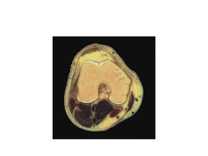
Figure 2. 12. View of the distal femur. This view demonstrates the slightly thinner medial femoral condyle which also has more acute inclination than the lateral. The anterior prominence of the trochlear flare on the lateral aspect demonstrates an obvious, increased anterior/posterior dimension for the lateral femoral condyle. (Reprinted with permission from I. A. Kapandji: The Physiology of the Joints, Vol. Il, Churchill Livingstone. New York, 1970(5). )

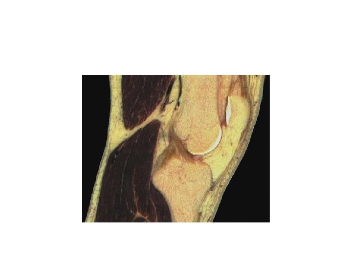
Figure 2. 13. (A) Diagrammatic sagittal section of the medial femoral condyle showing the radii of curvature. Anterior posterior dimension is smaller than that shown in B, which represents the lateral femoral condyle. (B) Lateral femoral condyle showing radii and centers of curvature and longer anterior posterior dimension. The overall forms of each femoral condyle is similar; however, the radii of curvature and general dimensions are dissimilar. (Reprinted with permission from I. A. Kapandji: The Physiology of the Joints, Vo. L II, Churchill Livingstone, New York, 1970(5). )

• 3 -D Morphology of the Distal Femur Viewed in Virtual Reality • (AAOS 2001 annual meeting - Scientific Exhibit No. SE 28) Donald G Eckhoff, MD, Denver, CO Thomas F Dwyer, MD, Denver, CO Joel M Bach, Ph. D, Aurora, CO Victor M Spitzer, Ph. D, Aurora, CO Karl D Reinig, Ph. D, Aurora, CO

• The morphologic shape of the distal femur dictates the shape, orientation and kinematics of prosthetic replacement in total knee arthroplasty. • Traditional prosthetic designs incorporate symmetric femoral condyles with a centered trochlear groove. Traditional surgical techniques center the femoral component to the distal femur and position it relative to variable bone landmarks. However, failure patterns documented in retrieval studies 13, 15, case series 9, and kinematic studies demonstrate how traditional design and surgical technique reflect a poor understanding of distal femoral morphology and knee kinematics.

• It has been shown that the flexion/extension (F/E) axis of the knee is fixed within the femur and that the articular surfaces of the condyles are circular in profile 11, 12. Ligament length patterns are significantly altered by abnormal axis alignment when using a hinged knee brace 14. It is expected that a malaligned femoral component would have the same effect in TKA. • The purpose of this exhibit is to demonstrate with conventional images and with interactive animations in virtual reality the three dimensional shape of the naturally asymmetric distal femur, illustrating the sulcus axis of the trochlear groove and flexion axis of the condyles relative to conventional axes (mechanical, anatomic, epicondylar & posterior condylar axes). Correlations between the morphologically determined rotation axes and experimentally determined kinematic axes are illustrated.

• Methods: Eighty five mummified cadaveric knees (fig. 1 below left) were measured with a stereotactic micrometer (fig. 2 below center). The location and orientation of the sulcus were obtained by repeated horizontal passes of the stereotactic stylus over the distal femur beginning at the top of the articular surface and progressing down to the intercondylar notch (fig. 3 below right). With each horizontal pass, the lowest depression of the trochlea (sulcus) was identified by the stereotactic stylus and the coordinates were recorded. After each horizontal pass, the stereotactic device was lowered by 2 mm to provide sequential horizontal tracings.

The stereotactic micrometer, originally designed to localize intra-cranial lesions in neurosurgery, was modified to hold cadaveric femora for topographical mapping of the condyles and trochlear groove (fig. 2 above center).

The stylus of the micrometer moves horizontally and vertically in millimeter increments to allow measures of depth in millimeters of the articular surface of the condyles and trochlea in the horizontal plane

The distal femora and proximal tibial computed tomography "cuts" were superimposed to measure relative translation and rotation. The proximal and distal femoral cuts were superimposed to measure femoral version (fig. 13 above right) 34 patients (34 knees) with anterior knee pain were measured by computed tomography and compared to 34 age matched normal knees (fig. 11 above right)

• The morphologic and biomechanical characteristics of the knee defined in these studies were measured in cyberspace and illustrated with a computer visualization program as an Interactive Anatomic Animation (IAA) in three additional cadaveric specimens. These three cadaveric knees were sectioned with CT into 0. 1 1. 0 mm slices, digitized, and reconstructed in virtual space (fig. 14 16 below).

Computer generated cylinders were "grown" within the confines of the articular surface of the distal femur to confirm and illustrate the cylindrical geometry of the condyles as well as demonstrate the position of the cylindrical axis relative to conventional axes (mechanical, anatomic, epicondylar & posterior condylar axes). (fig. 17 below)

• The sulcus of the trochlear groove lies lateral to the mid plane and is oriented between the mechanical and anatomic axes of the femur (fig. 18 below left, 19 below right).

sulcus of the trochlear groove lies lateral to the mid plane and is oriented between the mechanical and anatomic axes of the femur

• The sulcus (lowest point) is a near-linear depression in the trochlear groove that lies lateral to the midplane defined as the plane perpendicular to the posterior condylar axis. (fig. 18 above left) The sulcus is oriented between the traditional mechanical axis (line joining center of femoral head and center of knee) and • anatomic axis (center of femoral shaft). (fig. 19 above right)

sulcus of the trochlear groove lies lateral to the mid plane and is oriented between the mechanical and anatomic axes of the femur

• The cross sectional center of the femur lies medial and anterior to the cross sectional center of the tibia (fig. 20 below). • The cross-sectional centers of the distal femur and proximal tibia are not superimposed, but are translated 4+6 mm anteroposterior and 5+4 mm mediolateral in both normal and pathologic knees (ostheoarthritic and anterior knee pain). (fig. 20 above)

The cross sectional center of the femur lies medial and anterior to the cross sectional center of the tibia (fig. 20 below). The cross-sectional centers of the distal femur and proximal tibia are not superimposed, but are translated 4+6 mm anteroposterior and 5+4 mm mediolateral in both normal and pathologic knees (ostheoarthritic and anterior knee pain). (fig. 20 above)

One view of the Interactive Animation of the distal femur demonstrated in this exhibit illustrates the 3 -D relationship between the epicondylar axis (green line) and the "cylindrical axis" (red line) defined by the center of the cylinders which most closely reproduce the geometry of the condyles. (fig. 25 above)

• This study carefully documents the asymmetric morphologic features of the distal femur and correlates these features with the kinematics of the knee. • The location and orientation of the femoral sulcus is lateral to the midplane between the femoral condyles and oriented between the anatomic and mechanical axes of the femur. • The center of the femur in cross section is off set, medial and anterior, to the center of the tibia. • These asymmetric, off set morphologic features of distal femur should be incorporated in the design (fig. 26 below) and positioning of prosthetic replacements in the knee.

• These asymmetric, off set morphologic features of distal femur should be incorporated in the design (fig. 26 below) and positioning of prosthetic replacements in the knee.

• This study further documents • the asymmetric cylindrical shape of the condyles and • establishes the cylindrical axis of rotation of the condyles about which the tibia rotates. • The measured kinematic data supports the morphologic findings for a fixed, cylindrical flexion/extension axis of rotation. • This study provides kinematic and morphologic validation for a single cylindrical flexion/extension axis of the knee. • This scientific exhibit is the first to illustrate these observations in 3 D stereo using interactive animations and virtual reality. • (This Project has been funded in whole or in part with Federal funds from the National Library of Medicine under Contract No. N 01 LM 0 3507. )

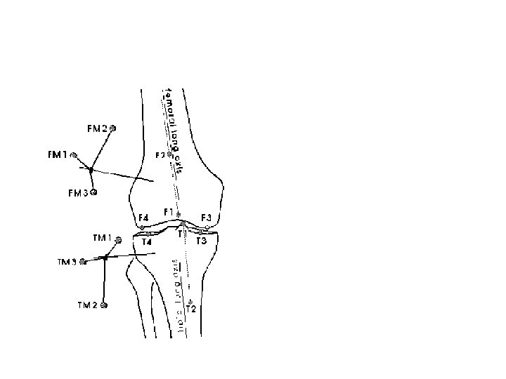
Figure 3. Centrally located points used in measures of alignment (as modified 9). The centers of the femoral intercondylar notch and tibial spines, respectively, denote the locations of the femoral axis distally and the tibial axis proximally in our recommended approach.

• PRINCIPLES AND MEASUREMENTS OF ALIGNMENT • From the anatomical and functional perspective, the orientation of the femur and tibia at the knee is best described in terms of the bones' mechanical axes. The orientation of these axes reflects alignment in stance, which may be neutral, varus (bowlegged), or valgus (knock kneed) (Figure 1).

Figure 1. Common frontal plane lower limb alignment patterns. A. Varus alignment: knee center is lateral to the LBA (HKA is negative). B. Neutral alignment: knee center is located on the LBA (HKA = 0°); femoral and tibial mechanical axes are colinear. C. Valgus alignment: knee center is medial to the LBA (HKA is positive). LBA: load bearing axis, HKA: hip knee ankle angle, FM: femoral mechanical axis, TM: tibial mechanical axis.

• The mechanical axis of the femur (FM) is located as a line from the center of the femoral head running distally to the mid condylar point between the cruciate ligaments 11. • In the case of the tibia, the mechanical axis (TM) is a line from the center of the tibial plateau (interspinous intercruciate midpoint) extending distally to the center of the tibial plafond 12 (Figure 2). • The angle between these 2 axes is the hip knee ankle (HKA) angle 1, 13. • In the neutrally aligned limb the HKA angle approaches 180°. At this point FM and TM are colinear, pass through the knee center, and are coincident with the load bearing axis, which is the line of ground reaction force passing from the ankle to the hip 1, 13 (Figure 1 B). • In varus the knee center is lateral to the load bearing axis (Figure 1 A), whereas in valgus the knee center is displaced medially 13, 14 (Figure 1 C). • As a convention the HKA angle may be expressed as its angular deviation from 180° (i. e. , HKA = 0° in neutral alignment). Varus deviations are negative and valgus deviations are positive. Our choice of varus as a negative value and valgus as positive was based on the general observations of a more serious problem of loading and damage in the varus knee.

Figure 2. Frontal plane angles in a limb with varus alignment. LBA: load bearing axis, CH: condylar hip angle, the angle of the femoral condylar tangent with respect to the femoral mechanical axis; varus negative, valgus positive. For the HKA measured as deviations from 90°. PA: plateau ankle angle, the angle between the tibial margin tangent and the tibial mechanical axis; varus negative, valgus positive. For the HKA measured as deviations from 90°. CP: condylar plateau angle: the angle between the femoral and tibial joint surface tangents; narrowing medially, negative, and laterally positive. HKA. Hip knee ankle angle: the angle between the femoral and tibial mechanical axes; varus negative, valgus positive. Measured as 180° equaling zero. FM: femoral mechanical axis, TM: tibial mechanical axis, FM FS: angle between the femoral mechanical axis and the femoral shaft axis.

• Limb alignment (HKA) depends both on long bone geometry and on the geometry of the articulating surfaces of the femur and tibia 1. In the course of knee arthritis, changes of alignment are usually ascribed to changes in the articulating geometry. Typically, focal erosion in the medial compartment leads to narrowing that, under load, displaces the knee center laterally (varus deformity; Figure 1 A). Similarly, narrowing of the lateral compartment imparts medial knee displacement (valgus deformity; Figure 1 C). But, on occasion, deformity of the femur and/or tibia also influences alignment. To understand the basis for alignment (and change thereof in the course of disease) it is crucial to be able to measure and document articular surface relationships and define limb bone morphology. Based on simple geometric analysis the following elements usefully define the geometry of the tibial and femoral surfaces and the angle between them when loaded in stance 1, 13 (Figure 2).

• 1. Condylar hip (CH): the angle of the femoral condylar tangent with respect to the FM axis; • 2. Plateau ankle (PA): the angle between the tibial margin tangent and the TM axis; • 3. Condylar plateau (CP): the angle between the femoral and tibial joint surface tangents. • Since HKA is expressed as degrees of deviation from 180°, CH and PA angles are expressed as degrees of deviation from 90°, negative for varus and positive for valgus. A joint space angle (CP) that narrows medially is designated varus (–) and laterally valgus (+). When these conventions are observed, the following relationship applies 1, 13: • HKA = CH + PA + CP

Figure 3. Centrally located points used in measures of alignment (as modified 9). The centers of the femoral intercondylar notch and tibial spines, respectively, denote the locations of the femoral axis distally and the tibial axis proximally in our recommended approach.

Tensegrity Knee Construction

. Tensegrity Knee Saddle Joint Two modified expanded octahedrons rotated 90 degrees to each other axially shows a remarkably close fit to the geometry of the knee.

Tensegrity Knee Construction In addition the patella is a tetrahedral shaped bone that nests in a gap between the femur and tibia, its position maintained by another saddle tension sling between the condyles of the femur. For the purposes of this simplified model the fibula is considered part of the tensegrity of the tibia.

Method of restructuring bone Document Type and Number: United States Patent 6719793 The method includes providing an implant structure having a calcium phosphate component, and stabilizing the implant adjacent the healthy bone until tissue can recover, bond to the implant and support the normal required loading. The implant structure provides morphological continuity and anatomical contact between the implant body and the adjacent healthy bone. The method further includes providing for physiological processes to maintain a healthy junction between the implant and the healthy bone. The method further includes controlling, guiding and directing the bone reconstruction process in surgical situations where healthy recovery would not otherwise occur.

• 1. A method of incorporating a prosthetic device into the skeletal structure of a human or animal for inducing bone repair and stabilizing a first and a second portion of damaged bone, comprising the steps of: providing an osteoceramic cylinder adapted to tightly fit into the intramedullary cavity of the damaged bone; positioning the osteoceramic cylinder inside the intramedullary cavities of the first and the second portions of damaged bone; and stabilizing the osteoceramic cylinder relative to the first and second portions of damaged bone. 2. The method of claim 1, wherein said step of stabilizing the osteoceramic cylinder further comprises positioning osteoceramic spacers on the outer surface of the osteoceramic cylinder. 3. The method of claim 1, wherein said step of stabilizing the osteoceramic cylinder further comprises connecting the osteoceramic cylinder to at least one of the first and second portions of damaged bone with one or more bone attachment means. 4. The method of claim 1, wherein the animal is an avian and the cylinder is hollow.

• FIELD OF THE INVENTION • This invention relates to a method of producing restructured bone, and more particularly to a method causing bone to bond to an implant containing a calcium phosphate component, and a method to control the restructuring of bone through the use of an implant containing calcium phosphate.

• Industrial Bioengineering Coordinator: Prof. Franco Maria Montevecchi •

• ENGINEERING IN SURGERY • Structural topology optimization methodologies applied to the study of boundary conditions in physiological femur and pelvis • The results obtained by structural analysis of hip arthroplasty models strongly depend on the correctness of the boundary conditions applied to the numerical model. • Structural topology optimization methodologies based on optimality criteria can be used to identify the most meaningful loading conditions and, for each of them, the correct set of applied forces able to justify the layout of the bone tissue of physiological skeletal element.

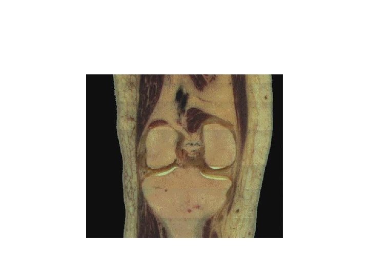
Examine the radiograph of the knee in a couple of views and identify the: • femur • medial condyle • lateral condyle • patella • tibia • medial condyle • lateral condyle • intercondylar eminence • head of fibula • neck of fibula

Examine the radiograph of the knee in a couple of views and identify the: • femur • medial condyle • lateral condyle • patella • tibia • medial condyle • lateral condyle • intercondylar eminence • head of fibula • neck of fibula

ENGINEERING IN ANATOMY AND SURGERY

Hvala na pažnji !!!

Hvala na pažnji !!!