Interconnect Performance Modeling Performance modeling Given an interconnect

Interconnect Performance Modeling

Performance modeling • Given an interconnect topology, routing, and other parameters, predict the interconnect performance – Throughput – Latency – Power consumption – Resilience (fault tolerance properties)

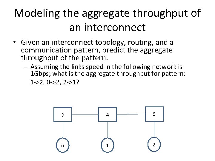
Modeling the aggregate throughput of an interconnect • Given an interconnect topology, routing, and a communication pattern, predict the aggregate throughput of the pattern. – Assuming the links speed in the following network is 1 Gbps; what is the aggregate throughput for pattern: 1 ->2, 0 ->2, 2 ->1? 3 4 5 0 1 2

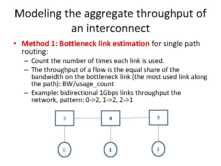
Modeling the aggregate throughput of an interconnect • Method 1: Bottleneck link estimation for single path routing: – Count the number of times each link is used. – The throughput of a flow is the equal share of the bandwidth on the bottleneck link (the most used link along the path): BW/usage_count – Example: bidirectional 1 Gbps links throughput the network, pattern: 0 ->2, 1 ->2, 2 ->1 3 4 5 0 1 2

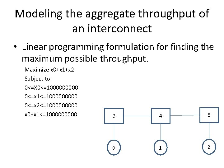
Modeling the aggregate throughput of an interconnect • Linear programming formulation for finding the maximum possible throughput. Maximize x 0+x 1+x 2 Subject to: 0<=X 0<=100000 0<=x 1<=100000 0<=x 2<=100000 x 0+x 1<=100000 3 4 5 0 1 2

Linear programming (LP) • Used extensively in solving networking modeling problems (and many other CS problems such as register allocation in compilers). • A linear programming is defined by – A set of variables – An optimization objective function (linear function of the set of variables) – A set of linear constraints (linear on the variables)

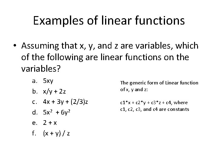
Examples of linear functions • Assuming that x, y, and z are variables, which of the following are linear functions on the variables? a. b. c. d. e. f. 5 xy x/y + 2 z 4 x + 3 y + (2/3)z 5 x 2 + 6 y 2 2+x (x + y) / z The generic form of Linear function of x, y and z: c 1*x + c 2*y + c 3*z + c 4, where c 1, c 2, c 3, and c 4 are constants

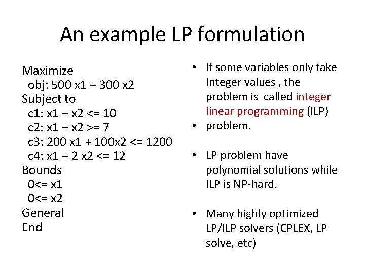
An example LP formulation Maximize obj: 500 x 1 + 300 x 2 Subject to c 1: x 1 + x 2 <= 10 c 2: x 1 + x 2 >= 7 c 3: 200 x 1 + 100 x 2 <= 1200 c 4: x 1 + 2 x 2 <= 12 Bounds 0<= x 1 0<= x 2 General End • If some variables only take Integer values , the problem is called integer linear programming (ILP) • problem. • LP problem have polynomial solutions while ILP is NP-hard. • Many highly optimized LP/ILP solvers (CPLEX, LP solve, etc)

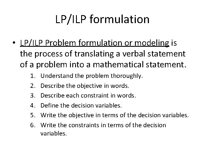
LP/ILP formulation • LP/ILP Problem formulation or modeling is the process of translating a verbal statement of a problem into a mathematical statement. 1. 2. 3. 4. 5. 6. Understand the problem thoroughly. Describe the objective in words. Describe each constraint in words. Define the decision variables. Write the objective in terms of the decision variables. Write the constraints in terms of the decision variables.

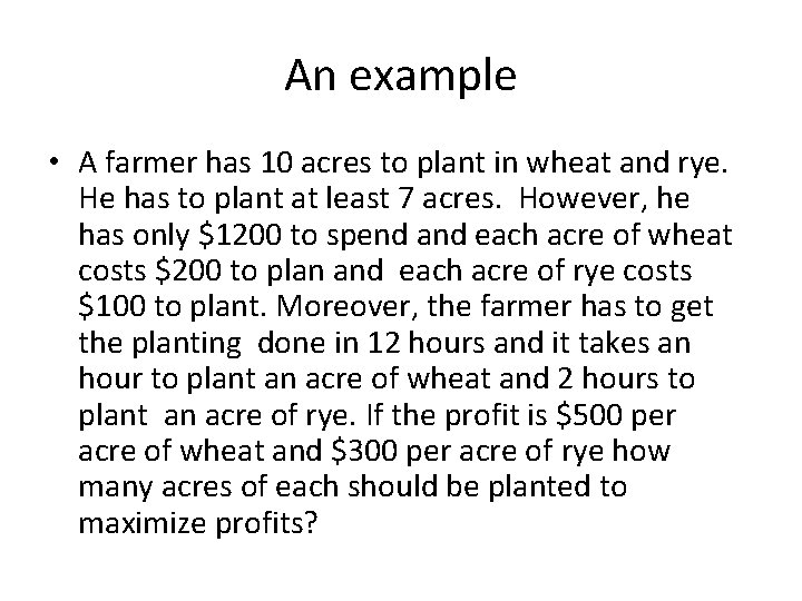
An example • A farmer has 10 acres to plant in wheat and rye. He has to plant at least 7 acres. However, he has only $1200 to spend and each acre of wheat costs $200 to plan and each acre of rye costs $100 to plant. Moreover, the farmer has to get the planting done in 12 hours and it takes an hour to plant an acre of wheat and 2 hours to plant an acre of rye. If the profit is $500 per acre of wheat and $300 per acre of rye how many acres of each should be planted to maximize profits?

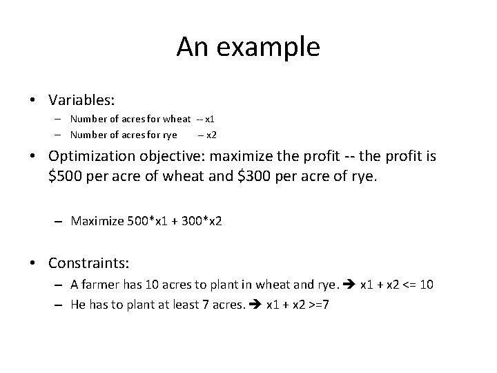
An example • Variables: – Number of acres for wheat -- x 1 – Number of acres for rye -- x 2 • Optimization objective: maximize the profit -- the profit is $500 per acre of wheat and $300 per acre of rye. – Maximize 500*x 1 + 300*x 2 • Constraints: – A farmer has 10 acres to plant in wheat and rye. x 1 + x 2 <= 10 – He has to plant at least 7 acres. x 1 + x 2 >=7

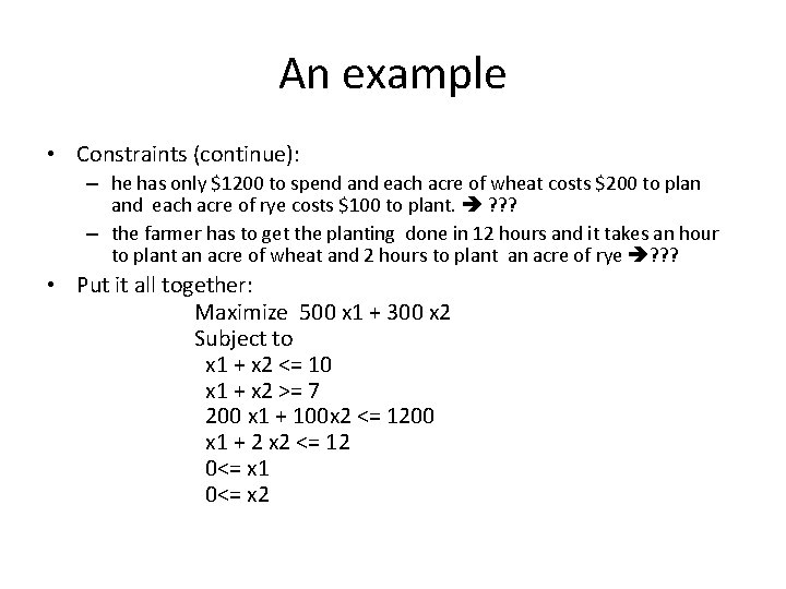
An example • Constraints (continue): – he has only $1200 to spend and each acre of wheat costs $200 to plan and each acre of rye costs $100 to plant. ? ? ? – the farmer has to get the planting done in 12 hours and it takes an hour to plant an acre of wheat and 2 hours to plant an acre of rye ? ? ? • Put it all together: Maximize 500 x 1 + 300 x 2 Subject to x 1 + x 2 <= 10 x 1 + x 2 >= 7 200 x 1 + 100 x 2 <= 1200 x 1 + 2 x 2 <= 12 0<= x 1 0<= x 2

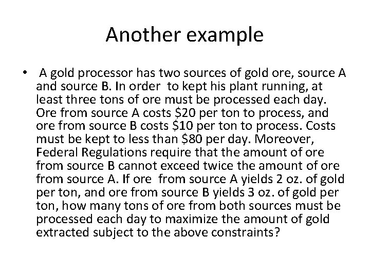
Another example • A gold processor has two sources of gold ore, source A and source B. In order to kept his plant running, at least three tons of ore must be processed each day. Ore from source A costs $20 per ton to process, and ore from source B costs $10 per ton to process. Costs must be kept to less than $80 per day. Moreover, Federal Regulations require that the amount of ore from source B cannot exceed twice the amount of ore from source A. If ore from source A yields 2 oz. of gold per ton, and ore from source B yields 3 oz. of gold per ton, how many tons of ore from both sources must be processed each day to maximize the amount of gold extracted subject to the above constraints?

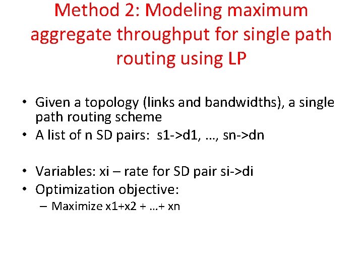
Method 2: Modeling maximum aggregate throughput for single path routing using LP • Given a topology (links and bandwidths), a single path routing scheme • A list of n SD pairs: s 1 ->d 1, …, sn->dn • Variables: xi – rate for SD pair si->di • Optimization objective: – Maximize x 1+x 2 + …+ xn

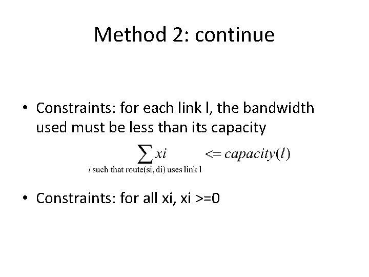
Method 2: continue • Constraints: for each link l, the bandwidth used must be less than its capacity • Constraints: for all xi, xi >=0

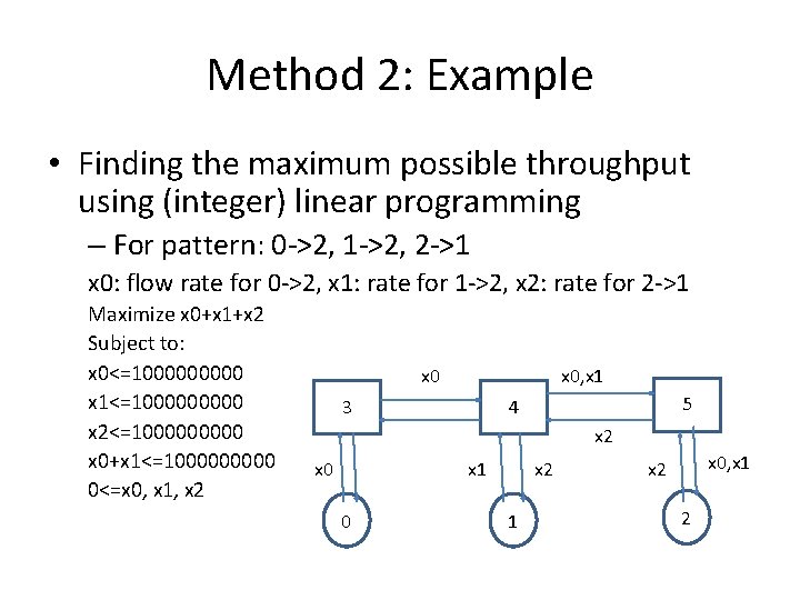
Method 2: Example • Finding the maximum possible throughput using (integer) linear programming – For pattern: 0 ->2, 1 ->2, 2 ->1 x 0: flow rate for 0 ->2, x 1: rate for 1 ->2, x 2: rate for 2 ->1 Maximize x 0+x 1+x 2 Subject to: x 0<=100000 x 1<=100000 x 2<=100000 x 0+x 1<=100000 0<=x 0, x 1, x 2 x 0, x 1 3 5 4 x 2 x 0 x 1 0 x 2 1 x 0, x 1 x 2 2

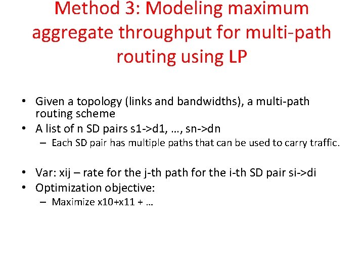
Method 3: Modeling maximum aggregate throughput for multi-path routing using LP • Given a topology (links and bandwidths), a multi-path routing scheme • A list of n SD pairs s 1 ->d 1, …, sn->dn – Each SD pair has multiple paths that can be used to carry traffic. • Var: xij – rate for the j-th path for the i-th SD pair si->di • Optimization objective: – Maximize x 10+x 11 + …

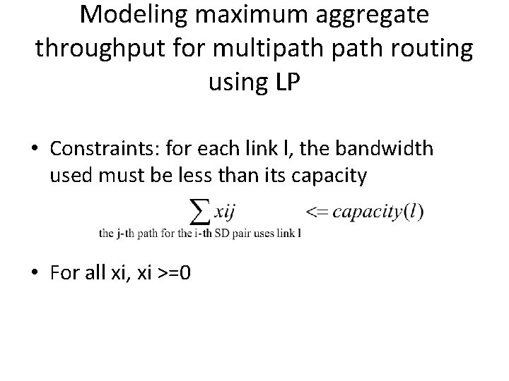
Modeling maximum aggregate throughput for multipath routing using LP • Constraints: for each link l, the bandwidth used must be less than its capacity • For all xi, xi >=0

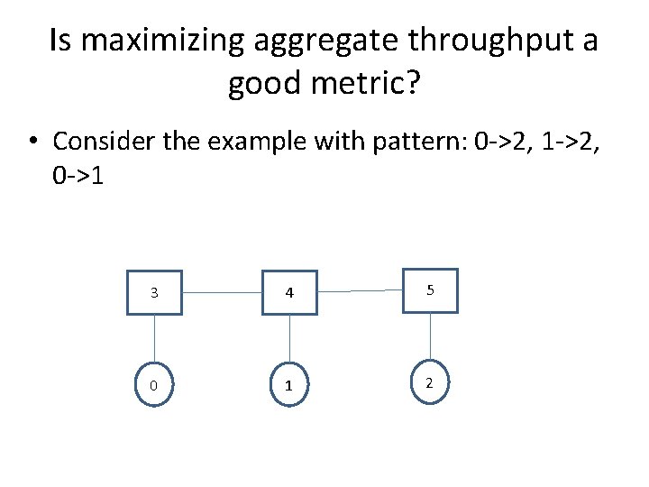
Is maximizing aggregate throughput a good metric? • Consider the example with pattern: 0 ->2, 1 ->2, 0 ->1 3 4 5 0 1 2

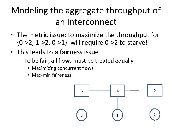
Modeling the aggregate throughput of an interconnect • The metric issue: to maximize throughput for {0 ->2, 1 ->2, 0 ->1} will require 0 ->2 to starve!! • This leads to a fairness issue – To be fair, all flows must be treated equally • Maximizing concurrent flows • Max-min faireness 3 4 5 0 1 2

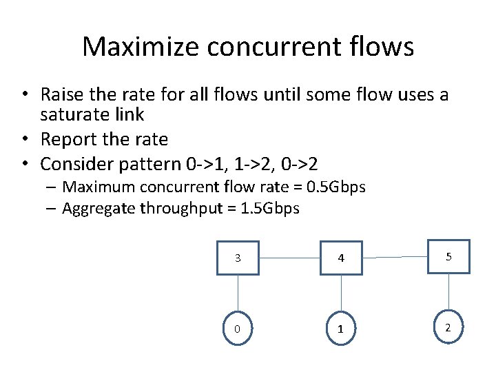
Maximize concurrent flows • Raise the rate for all flows until some flow uses a saturate link • Report the rate • Consider pattern 0 ->1, 1 ->2, 0 ->2 – Maximum concurrent flow rate = 0. 5 Gbps – Aggregate throughput = 1. 5 Gbps 3 4 5 0 1 2

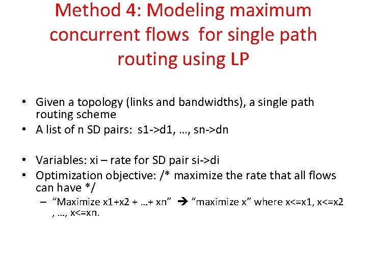
Method 4: Modeling maximum concurrent flows for single path routing using LP • Given a topology (links and bandwidths), a single path routing scheme • A list of n SD pairs: s 1 ->d 1, …, sn->dn • Variables: xi – rate for SD pair si->di • Optimization objective: /* maximize the rate that all flows can have */ – “Maximize x 1+x 2 + …+ xn” “maximize x” where x<=x 1, x<=x 2 , …, x<=xn.

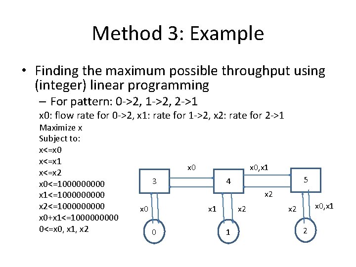
Method 3: Example • Finding the maximum possible throughput using (integer) linear programming – For pattern: 0 ->2, 1 ->2, 2 ->1 x 0: flow rate for 0 ->2, x 1: rate for 1 ->2, x 2: rate for 2 ->1 Maximize x Subject to: x<=x 0 x<=x 1 x<=x 2 x 0<=100000 x 1<=100000 x 2<=100000 x 0+x 1<=100000 0<=x 0, x 1, x 2 x 0, x 1 3 5 4 x 2 x 0 x 1 0 x 2 1 x 0, x 1 x 2 2

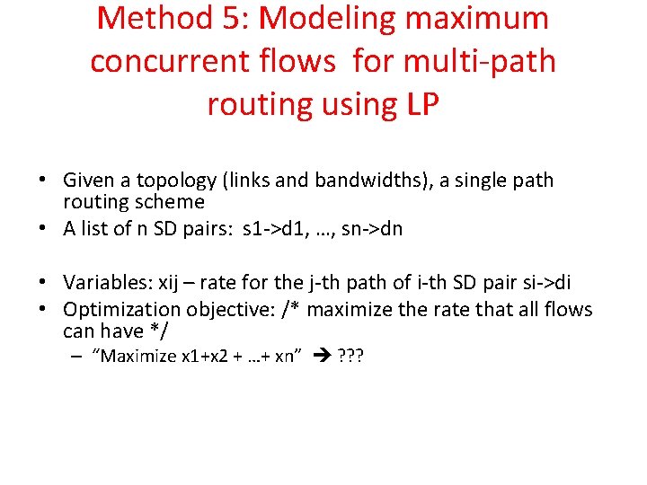
Method 5: Modeling maximum concurrent flows for multi-path routing using LP • Given a topology (links and bandwidths), a single path routing scheme • A list of n SD pairs: s 1 ->d 1, …, sn->dn • Variables: xij – rate for the j-th path of i-th SD pair si->di • Optimization objective: /* maximize the rate that all flows can have */ – “Maximize x 1+x 2 + …+ xn” ? ? ?

Max-min fairness • Given a network and a set of active users (identified by source destination pairs), what is the optimal rate allocation for these users? – Maximize aggregate throughput – Fairness among all users.

Modeling maximum stationary aggregate throughput • How to define fairness? – “Any session is entitled to as much network use as is any other, ” – “Unless some sessions can use more without hurting others. ” – This is the intuition of Max-Min fairness • Other fairness definitions – Network usage should depend on the resource consumption by the session.

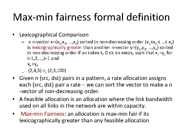
Max-min fairness formal definition • Lexicographical Comparison – a n-vector x=(x 1, x 2, …, xn) sorted in non-decreasing order (x 1≤x 2 ≤ …≤ xn) is lexicographically greater than another n-vector y=(y 1, y 2, …, yn) sorted in non-decreasing order if an index k, 0 ≤k ≤n exists, such that xi =yi, for i=1, 2, …, k-1 and xk >yk – (2, 4, 5) >L (2, 3, 100) • Given n (src, dst) pairs in a pattern, a rate allocation assigns each (src, dst) pair a rate – we can sort the vector to make a n -vector of non-decreasing order. • A feasible allocation is an allocation where the link bandwidth used on all links in the network are within capacity. • Max-min Fairness: an allocation is max-min fair if its lexicographically greater than any feasible allocation

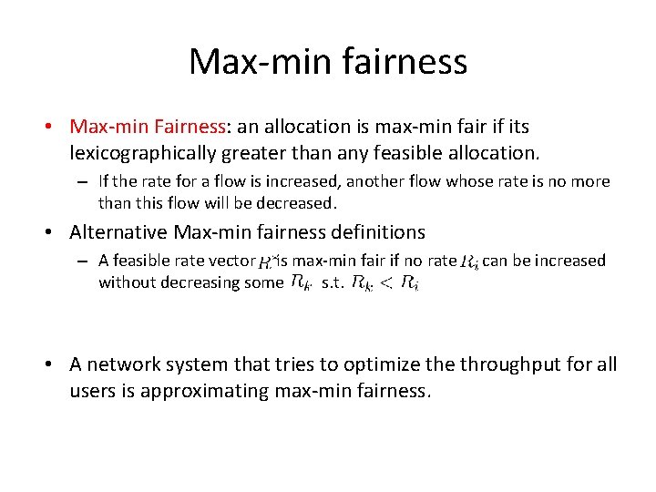
Max-min fairness • Max-min Fairness: an allocation is max-min fair if its lexicographically greater than any feasible allocation. – If the rate for a flow is increased, another flow whose rate is no more than this flow will be decreased. • Alternative Max-min fairness definitions – A feasible rate vector is max-min fair if no rate without decreasing some s. t. can be increased • A network system that tries to optimize throughput for all users is approximating max-min fairness.

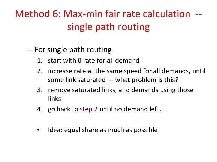
Method 6: Max-min fair rate calculation -single path routing – For single path routing: 1. start with 0 rate for all demand 2. increase rate at the same speed for all demands, until some link saturated -- what problem is this? 3. remove saturated links, and demands using those links 4. go back to step 2 until no demand left. • Idea: equal share as much as possible

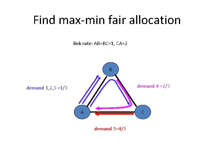
Find max-min fair allocation link rate: AB=BC=1, CA=2 B demand 4 =2/3 demand 1, 2, 3 =1/3 A C demand 5=4/3

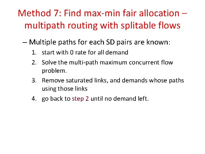
Method 7: Find max-min fair allocation – multipath routing with splitable flows – Multiple paths for each SD pairs are known: 1. start with 0 rate for all demand 2. Solve the multi-path maximum concurrent flow problem. 3. Remove saturated links, and demands whose paths using those links 4. go back to step 2 until no demand left.

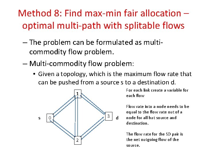
Method 8: Find max-min fair allocation – optimal multi-path with splitable flows – The problem can be formulated as multicommodity flow problem. – Multi-commodity flow problem: • Given a topology, which is the maximum flow rate that can be pushed from a source s to a destination d. For each link create a variable for each flow 1 s 3 0 2 d Flow rate into a node needs to be equal to the flow rate out of a node for all but source and destination. The flow rate for the SD pair is the net outgoing flow of the source.

Method 8: Find max-min fair allocation – optimal multi-path with splitable flows – The problem can be formulated as multicommodity flow problem. – Same logical as Method 7 with a different max concurrent flow problem to solve in every step. – See this paper be more details: • Nace, Dritan and Nhat Doan, Linh and Klopfenstein, Olivier and Bashllari, Alfred, “Max-min Fairness in Multi -commodity Flows”, Computers and Operations Research, 35(2): 557 -573, February 2008.