Lecture 25 Networks Interconnect Networks on a Chip

Lecture 25: Networks & Interconnect Networks on a Chip Prepared by: Professor David A. Patterson Professor Bill Dally (Stanford) Edited and presented by : Prof. Jan Rabaey Computer Science 252, Spring 2000 JR. S 00 1

Project Presentations Next Week • The Good News: No presentations on Tu faculty retreat – time for contemplation • The Bad News: A monster session on Th: 26 pm (? ) • Each group gets 15 minutes (12’ + 3) – Use overhead or mail in powerpoint a day in advance • Conference style presentation • Be concise JR. S 00 2

Review: Interconnections • Communication between computing elements • Protocols to cover normal and abnormal events • Performance issues: HW & SW overhead, interconnect latency, bisection BW • Media sets cost, distance • HW and SW Interface to computer affects overhead, latency, bandwidth JR. S 00 3

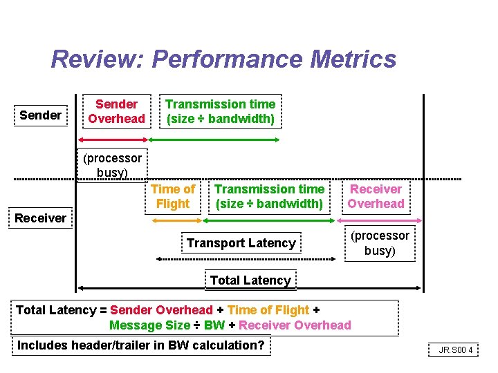
Review: Performance Metrics Sender Overhead Transmission time (size ÷ bandwidth) (processor busy) Time of Flight Transmission time (size ÷ bandwidth) Receiver Overhead Receiver Transport Latency (processor busy) Total Latency = Sender Overhead + Time of Flight + Message Size ÷ BW + Receiver Overhead Includes header/trailer in BW calculation? JR. S 00 4

Interconnect Issues • • Performance Measures Interface Issues Network Media Connecting Multiple Computers JR. S 00 5

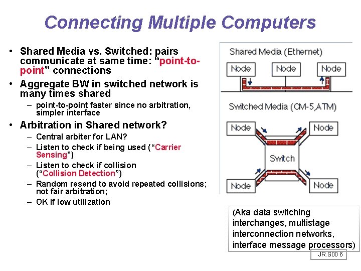
Connecting Multiple Computers • Shared Media vs. Switched: pairs communicate at same time: “point-topoint” connections • Aggregate BW in switched network is many times shared – point-to-point faster since no arbitration, simpler interface • Arbitration in Shared network? – Central arbiter for LAN? – Listen to check if being used (“Carrier Sensing”) – Listen to check if collision (“Collision Detection”) – Random resend to avoid repeated collisions; not fair arbitration; – OK if low utilization (Aka data switching interchanges, multistage interconnection networks, interface message processors) JR. S 00 6

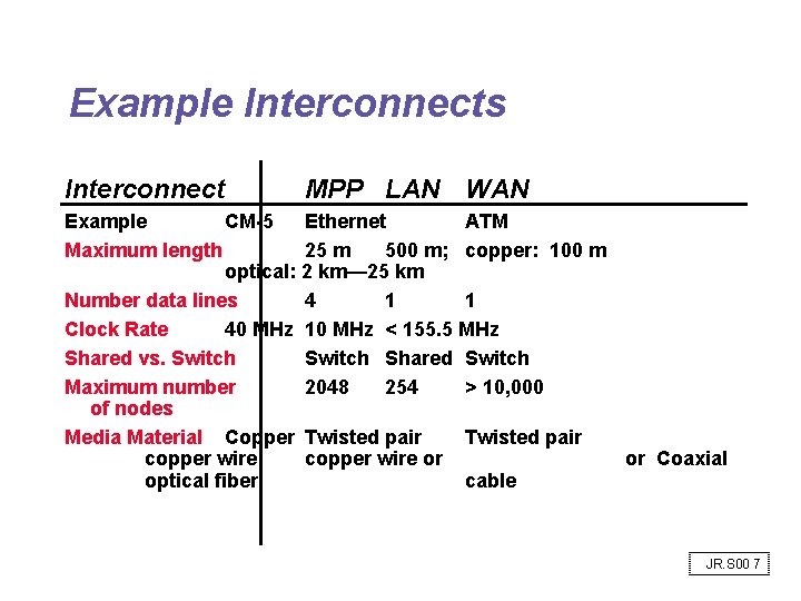
Example Interconnects Interconnect MPP LAN WAN Example CM-5 Ethernet ATM Maximum length 25 m 500 m; copper: 100 m optical: 2 km— 25 km Number data lines 4 1 1 Clock Rate 40 MHz 10 MHz < 155. 5 MHz Shared vs. Switch Shared Switch Maximum number 2048 254 > 10, 000 of nodes Media Material Copper Twisted pair copper wire or or Coaxial optical fiber cable JR. S 00 7

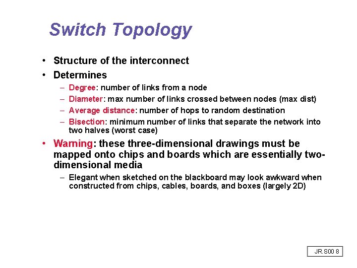
Switch Topology • Structure of the interconnect • Determines – – Degree: number of links from a node Diameter: max number of links crossed between nodes (max dist) Average distance: number of hops to random destination Bisection: minimum number of links that separate the network into two halves (worst case) • Warning: these three-dimensional drawings must be mapped onto chips and boards which are essentially twodimensional media – Elegant when sketched on the blackboard may look awkward when constructed from chips, cables, boards, and boxes (largely 2 D) JR. S 00 8

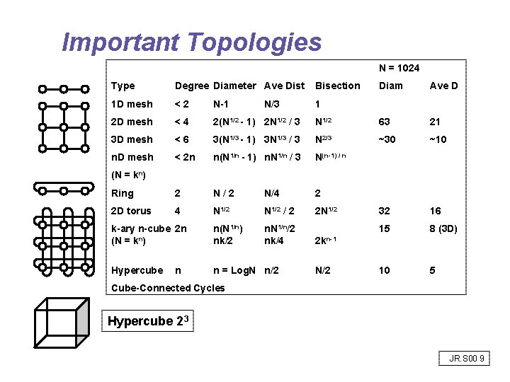
Important Topologies N = 1024 Type Degree Diameter Ave Dist Bisection Diam Ave D 1 D mesh <2 N-1 1 2 D mesh <4 2(N 1/2 - 1) 2 N 1/2 / 3 N 1/2 63 21 3 D mesh <6 3(N 1/3 - 1) 3 N 1/3 / 3 N 2/3 ~30 ~10 n. D mesh < 2 n n(N 1/n - 1) n. N 1/n / 3 N(n-1) / n Ring 2 N/4 2 2 D torus 4 N 1/2 / 2 2 N 1/2 32 16 k-ary n-cube 2 n (N = kn) n(N 1/n) nk/2 n. N 1/n/2 nk/4 15 8 (3 D) 2 kn-1 Hypercube n = Log. N n/2 10 5 N/3 (N = kn) n N/2 Cube-Connected Cycles Hypercube 23 JR. S 00 9

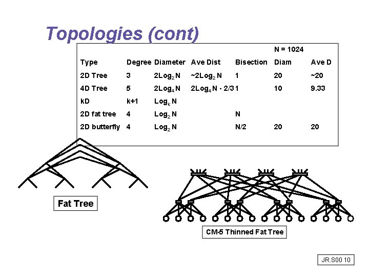
Topologies (cont) N = 1024 Type Degree Diameter Ave Dist Bisection Diam Ave D 2 D Tree 3 2 Log 2 N ~2 Log 2 N 1 20 ~20 4 D Tree 5 2 Log 4 N - 2/3 1 10 9. 33 k. D k+1 Logk N 2 D fat tree 4 Log 2 N N 2 D butterfly 4 Log 2 N N/2 20 20 Fat Tree CM-5 Thinned Fat Tree JR. S 00 10

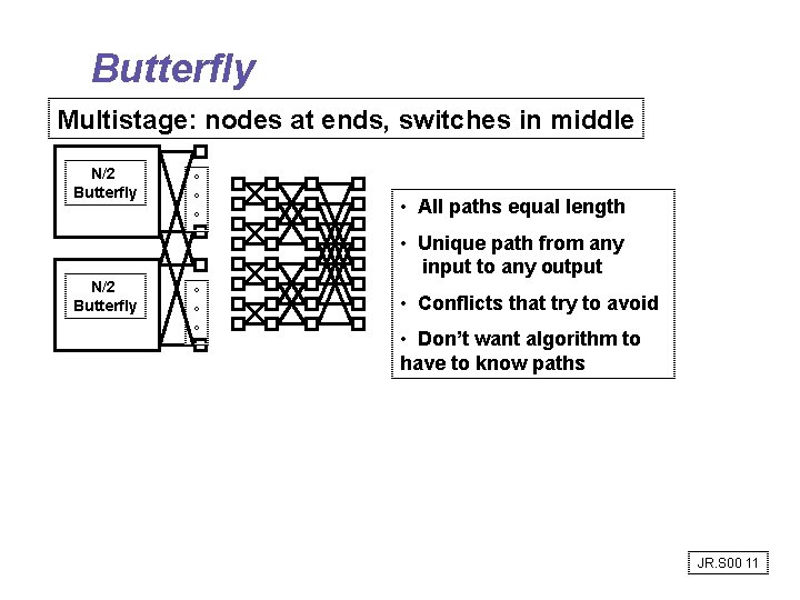
Butterfly Multistage: nodes at ends, switches in middle N/2 Butterfly ° ° ° • All paths equal length • Unique path from any input to any output N/2 Butterfly ° ° ° • Conflicts that try to avoid • Don’t want algorithm to have to know paths JR. S 00 11

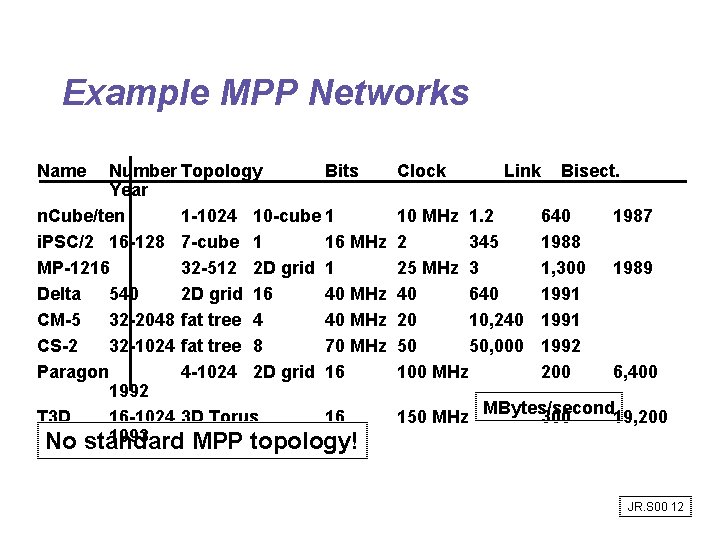
Example MPP Networks Name Number Topology Bits Year n. Cube/ten 1 -1024 10 -cube 1 i. PSC/2 16 -128 7 -cube 1 16 MHz MP-1216 32 -512 2 D grid 1 Delta 540 2 D grid 16 40 MHz CM-5 32 -2048 fat tree 4 40 MHz CS-2 32 -1024 fat tree 8 70 MHz Paragon 4 -1024 2 D grid 16 1992 T 3 D 16 -1024 3 D Torus 16 1993 No standard MPP topology! Clock Link 10 MHz 1. 2 2 345 25 MHz 3 40 640 20 10, 240 50 50, 000 100 MHz 150 MHz Bisect. 640 1988 1, 300 1991 1992 200 1987 1989 6, 400 MBytes/second 300 19, 200 JR. S 00 12

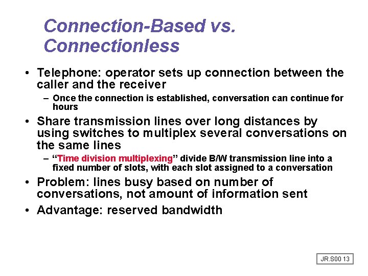
Connection-Based vs. Connectionless • Telephone: operator sets up connection between the caller and the receiver – Once the connection is established, conversation can continue for hours • Share transmission lines over long distances by using switches to multiplex several conversations on the same lines – “Time division multiplexing” divide B/W transmission line into a fixed number of slots, with each slot assigned to a conversation • Problem: lines busy based on number of conversations, not amount of information sent • Advantage: reserved bandwidth JR. S 00 13

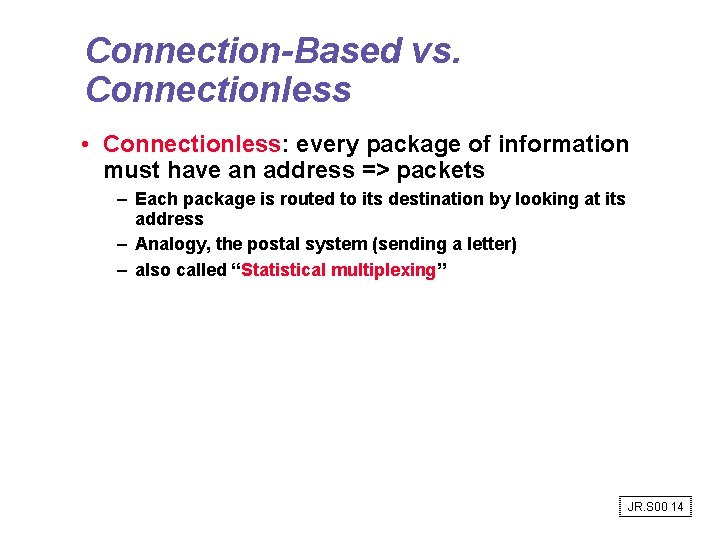
Connection-Based vs. Connectionless • Connectionless: every package of information must have an address => packets – Each package is routed to its destination by looking at its address – Analogy, the postal system (sending a letter) – also called “Statistical multiplexing” JR. S 00 14

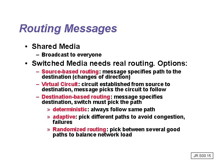
Routing Messages • Shared Media – Broadcast to everyone • Switched Media needs real routing. Options: – Source-based routing: message specifies path to the destination (changes of direction) – Virtual Circuit: circuit established from source to destination, message picks the circuit to follow – Destination-based routing: message specifies destination, switch must pick the path » deterministic: always follow same path » adaptive: pick different paths to avoid congestion, failures » Randomized routing: pick between several good paths to balance network load JR. S 00 15

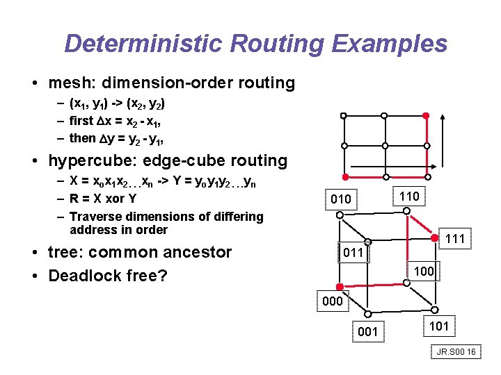
Deterministic Routing Examples • mesh: dimension-order routing – (x 1, y 1) -> (x 2, y 2) – first x = x 2 - x 1, – then y = y 2 - y 1, • hypercube: edge-cube routing – X = xox 1 x 2. . . xn -> Y = yoy 1 y 2. . . yn – R = X xor Y – Traverse dimensions of differing address in order • tree: common ancestor • Deadlock free? 110 010 111 011 100 001 101 JR. S 00 16

Store and Forward vs. Cut-Through • Store-and-forward policy: each switch waits for the full packet to arrive in switch before sending to the next switch (good for WAN) • Cut-through routing and worm hole routing: switch examines the header, decides where to send the message, and then starts forwarding it immediately – In worm hole routing, when head of message is blocked, message stays strung out over the network, potentially blocking other messages (needs only buffer the piece of the packet that is sent between switches). CM-5 uses it, with each switch buffer being 4 bits per port. – Cut through routing lets the tail continue when head is blocked, accordioning the whole message into a single switch. (Requires a buffer large enough to hold the largest packet). JR. S 00 17

Store and Forward vs. Cut-Through • Advantage – Latency reduces from function of: number of intermediate switches X by the size of the packet to time for 1 st part of the packet to negotiate the switches + the packet size ÷ interconnect BW JR. S 00 18

Congestion Control • Packet switched networks do not reserve bandwidth; this leads to contention (connection based limits input) • Solution: prevent packets from entering until contention is reduced (e. g. , freeway on-ramp metering lights) • Options: – Packet discarding: If packet arrives at switch and no room in buffer, packet is discarded (e. g. , UDP) – Flow control: between pairs of receivers and senders; use feedback to tell sender when allowed to send next packet » Back-pressure: separate wires to tell to stop » Window: give original sender right to send N packets before getting permission to send more; overlaps latency of interconnection with overhead to send & receive packet (e. g. , TCP), adjustable window – Choke packets: aka “rate-based”; Each packet received by busy switch in warning state sent back to the source via choke packet. Source reduces traffic to that destination by a fixed % (e. g. , ATM) JR. S 00 19

Practical Issues for Interconnection Networks • Standardization advantages: – low cost (components used repeatedly) – stability (many suppliers to chose from) • Standardization disadvantages: – Time for committees to agree – When to standardize? » Before anything built? => Committee does design? » Too early suppresses innovation • Perfect interconnect vs. Fault Tolerant? – Will SW crash on single node prevent communication? (MPP typically assume perfect) • Reliability (vs. availability) of interconnect JR. S 00 20

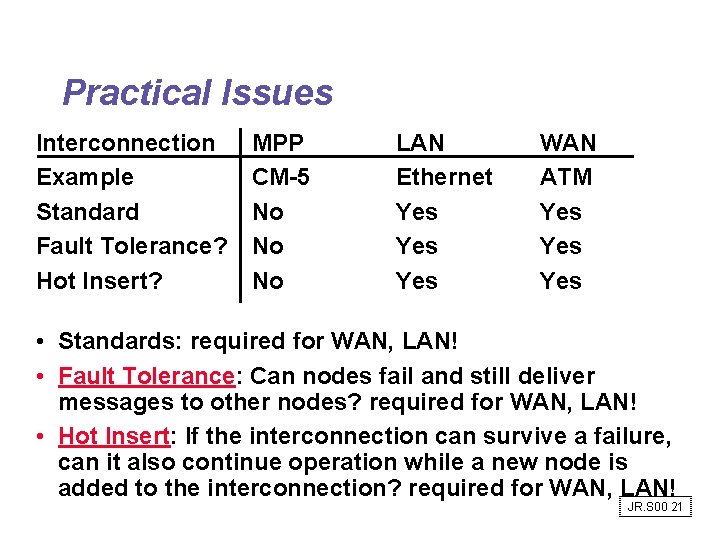
Practical Issues Interconnection Example Standard Fault Tolerance? Hot Insert? MPP CM-5 No No No LAN Ethernet Yes Yes WAN ATM Yes Yes • Standards: required for WAN, LAN! • Fault Tolerance: Can nodes fail and still deliver messages to other nodes? required for WAN, LAN! • Hot Insert: If the interconnection can survive a failure, can it also continue operation while a new node is added to the interconnection? required for WAN, LAN! JR. S 00 21

Networks on a Chip JR. S 00 22

Message • Interconnect-oriented architecture can reduce the demand for interconnect bandwidth and the effect of interconnect latency by an order of magnitude through – locality - eliminate global structures – hierarchy - expose locality in register architecture – networking - share the wires JR. S 00 23

Outline • Technology constraints • On-chip interconnection networks – regular wiring - well characterized – optimized circuits – efficient usage • Placement and Migration • Architecture for locality JR. S 00 24

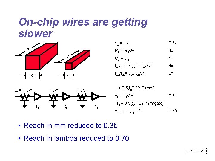
On-chip wires are getting slower y y x 1 x 2 tw = RCy 2 x 2 = s x 1 0. 5 x R 2 = R 1/s 2 4 x C 2 = C 1 1 x tw 2 = R 2 C 2 y 2 = tw 1/s 2 4 x tw 2/tg 2= tw 1/(tg 1 s 3) 8 x v = 0. 5(tg. RC)-1/2 (m/s) RCy 2 v 2 = v 1 s 1/2 tg tg tg 0. 7 x vtg = 0. 5(tg/RC)1/2 (m/gate) v 2 tg 2 = v 1 tg 1 s 3/2 0. 35 x • Reach in mm reduced to 0. 35 • Reach in lambda reduced to 0. 70 JR. S 00 25

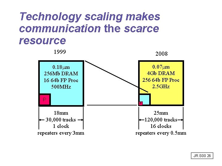
Technology scaling makes communication the scarce resource 1999 2008 0. 18 mm 256 Mb DRAM 16 64 b FP Proc 500 MHz 0. 07 mm 4 Gb DRAM 256 64 b FP Proc 2. 5 GHz P 18 mm 30, 000 tracks 1 clock repeaters every 3 mm P 25 mm 120, 000 tracks 16 clocks repeaters every 0. 5 mm JR. S 00 26

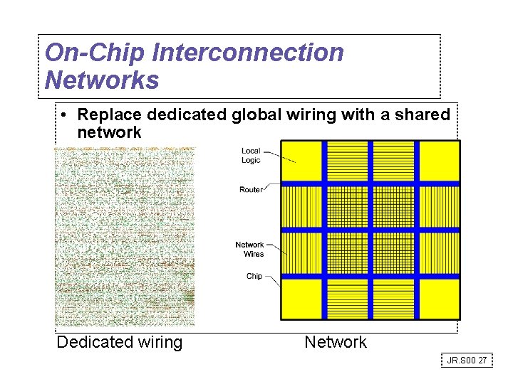
On-Chip Interconnection Networks • Replace dedicated global wiring with a shared network Dedicated wiring Network JR. S 00 27

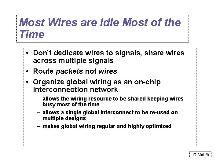
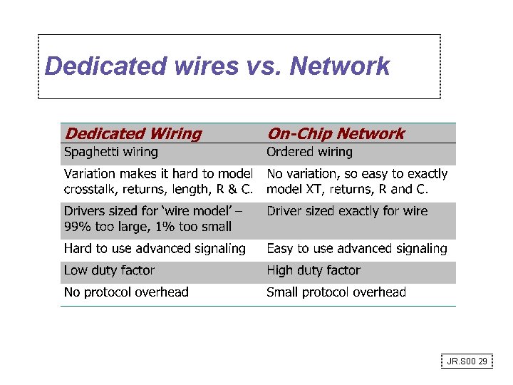
Most Wires are Idle Most of the Time • Don’t dedicate wires to signals, share wires across multiple signals • Route packets not wires • Organize global wiring as an on-chip interconnection network – allows the wiring resource to be shared keeping wires busy most of the time – allows a single global interconnect to be re-used on multiple designs – makes global wiring regular and highly optimized JR. S 00 28

Dedicated wires vs. Network JR. S 00 29

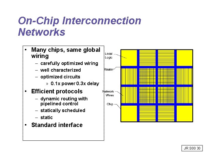
On-Chip Interconnection Networks • Many chips, same global wiring – carefully optimized wiring – well characterized – optimized circuits » 0. 1 x power 0. 3 x delay • Efficient protocols – dynamic routing with pipelined control – statically scheduled – static • Standard interface JR. S 00 30

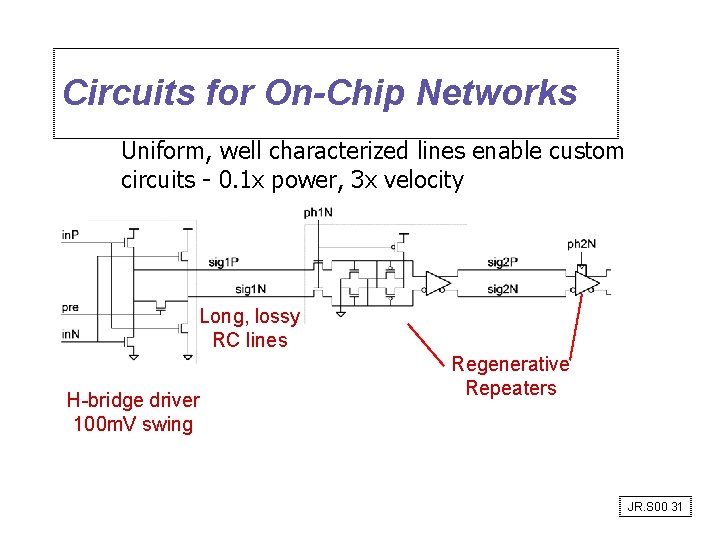
Circuits for On-Chip Networks Uniform, well characterized lines enable custom circuits - 0. 1 x power, 3 x velocity Long, lossy RC lines H-bridge driver 100 m. V swing Regenerative Repeaters JR. S 00 31

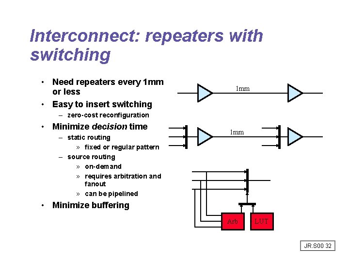
Interconnect: repeaters with switching • Need repeaters every 1 mm or less • Easy to insert switching 1 mm – zero-cost reconfiguration • Minimize decision time – static routing » fixed or regular pattern – source routing » on-demand » requires arbitration and fanout » can be pipelined 1 mm • Minimize buffering Arb LUT JR. S 00 32

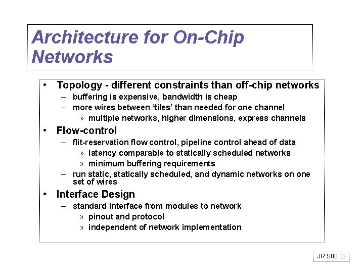
Architecture for On-Chip Networks • Topology - different constraints than off-chip networks – buffering is expensive, bandwidth is cheap – more wires between ‘tiles’ than needed for one channel » multiple networks, higher dimensions, express channels • Flow-control – flit-reservation flow control, pipeline control ahead of data » latency comparable to statically scheduled networks » minimum buffering requirements – run static, statically scheduled, and dynamic networks on one set of wires • Interface Design – standard interface from modules to network » pinout and protocol » independent of network implementation JR. S 00 33

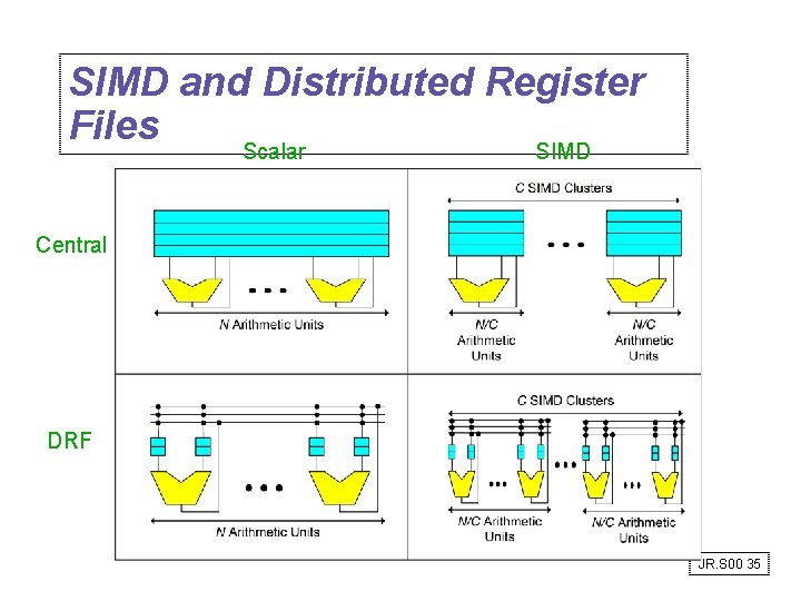
SIMD and Distributed Register Files Scalar SIMD Central DRF JR. S 00 35

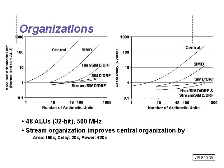
Organizations • 48 ALUs (32 -bit), 500 MHz • Stream organization improves central organization by Area: 195 x, Delay: 20 x, Power: 430 x JR. S 00 36

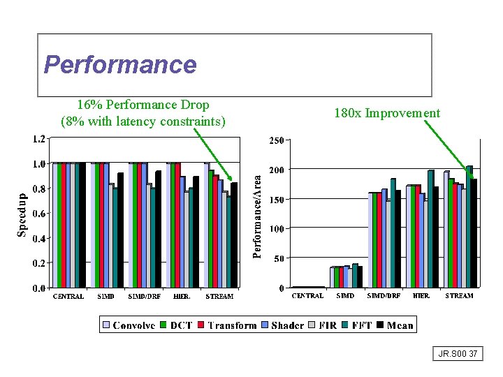
Performance 16% Performance Drop (8% with latency constraints) 180 x Improvement JR. S 00 37

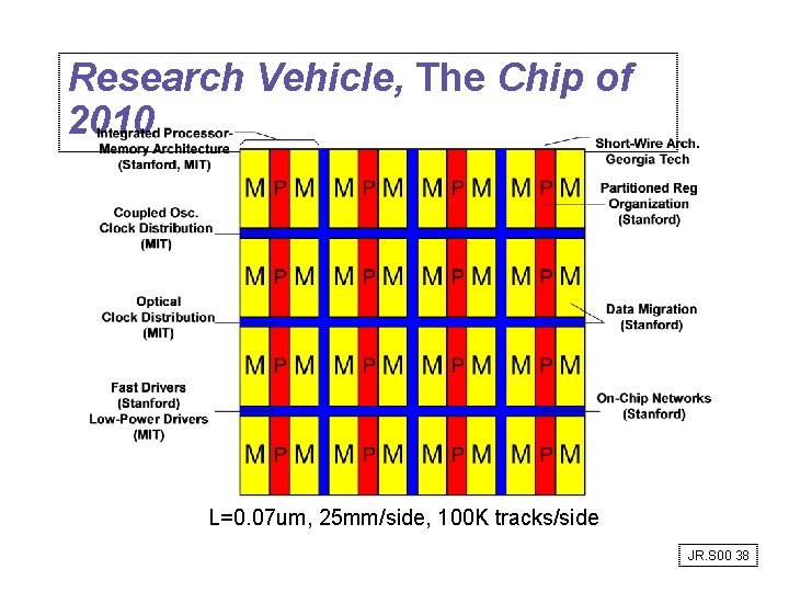
Research Vehicle, The Chip of 2010 L=0. 07 um, 25 mm/side, 100 K tracks/side JR. S 00 38

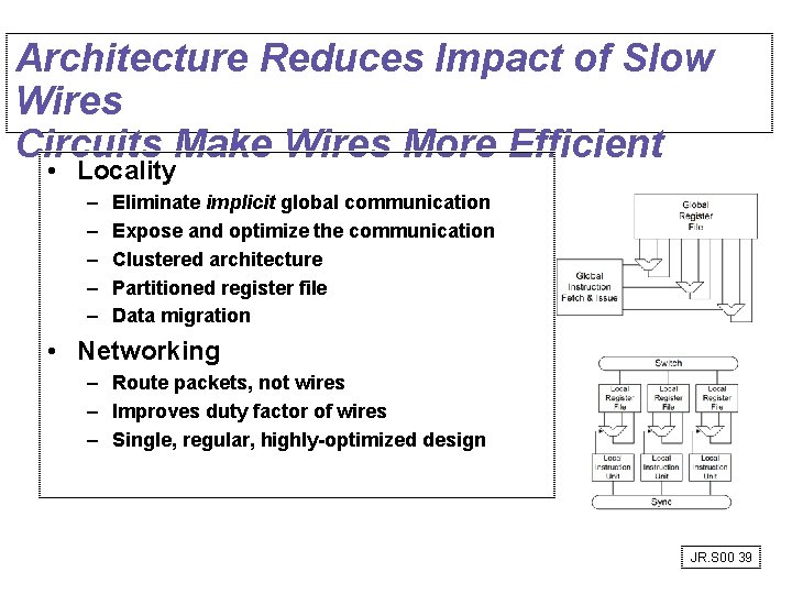
Architecture Reduces Impact of Slow Wires Circuits Make Wires More Efficient • Locality – – – Eliminate implicit global communication Expose and optimize the communication Clustered architecture Partitioned register file Data migration • Networking – Route packets, not wires – Improves duty factor of wires – Single, regular, highly-optimized design JR. S 00 39

Protocols: HW/SW Interface • Internetworking: allows computers on independent and incompatible networks to communicate reliably and efficiently; – Enabling technologies: SW standards that allow reliable communications without reliable networks – Hierarchy of SW layers, giving each layer responsibility for portion of overall communications task, called protocol families or protocol suites • Transmission Control Protocol/Internet Protocol (TCP/IP) – This protocol family is the basis of the Internet – IP makes best effort to deliver; TCP guarantees delivery – TCP/IP used even when communicating locally: NFS uses IP even though communicating across homogeneous LAN JR. S 00 40

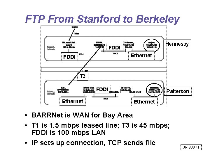
FTP From Stanford to Berkeley Hennessy FDDI Ethernet FDDI T 3 FDDI Ethernet Patterson Ethernet • BARRNet is WAN for Bay Area • T 1 is 1. 5 mbps leased line; T 3 is 45 mbps; FDDI is 100 mbps LAN • IP sets up connection, TCP sends file JR. S 00 41

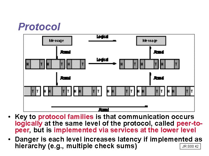
Protocol • Key to protocol families is that communication occurs logically at the same level of the protocol, called peer-topeer, but is implemented via services at the lower level • Danger is each level increases latency if implemented as JR. S 00 42 hierarchy (e. g. , multiple check sums)

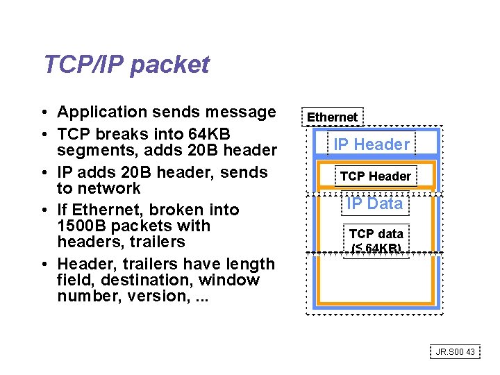
TCP/IP packet • Application sends message • TCP breaks into 64 KB segments, adds 20 B header • IP adds 20 B header, sends to network • If Ethernet, broken into 1500 B packets with headers, trailers • Header, trailers have length field, destination, window number, version, . . . Ethernet IP Header TCP Header IP Data TCP data (≤ 64 KB) JR. S 00 43

Example Networks • Ethernet: shared media 10 Mbit/s proposed in 1978, carrier sensing with expotential backoff on collision detection • 15 years with no improvement; higher BW? • Multiple Ethernets with devices to allow Ehternets to operate in parallel! • 10 Mbit Ethernet successors? – – – FDDI: shared media (too late) ATM (too late? ) Switched Ethernet 100 Mbit Ethernet (Fast Ethernet) Gigabit Ethernet JR. S 00 44

Connecting Networks • Bridges: connect LANs together, passing traffic from one side to another depending on the addresses in the packet. – operate at the Ethernet protocol level – usually simpler and cheaper than routers • Routers or Gateways: these devices connect LANs to WANs or WANs to WANs and resolve incompatible addressing. – Generally slower than bridges, they operate at the internetworking protocol (IP) level – Routers divide the interconnect into separate smaller subnets, which simplifies manageability and improves security • Cisco is major supplier; basically special purpose computers JR. S 00 45

Networking Summary • Protocols allow hetereogeneous networking • Protocols allow operation in the presense of failures • Routing issues: store and forward vs. cut through, congestion, . . . • Standardization key for LAN, WAN • Internetworking protocols used as LAN protocols => large overhead for LAN • Integrated circuit revolutionizing networks as well as processors JR. S 00 46