Images and Filters ECE P 596 Linda Shapiro

Images and Filters ECE P 596 Linda Shapiro

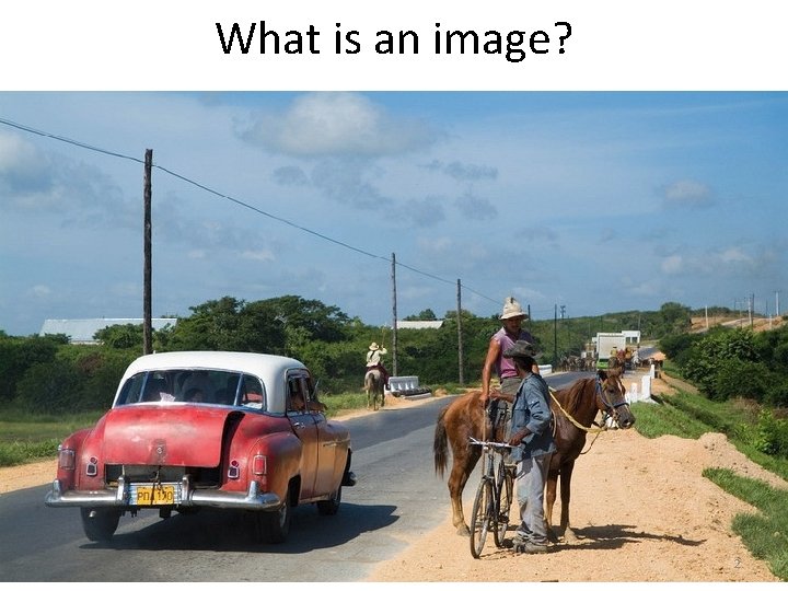
What is an image? 2

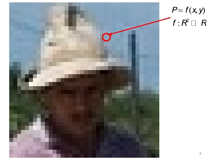
3

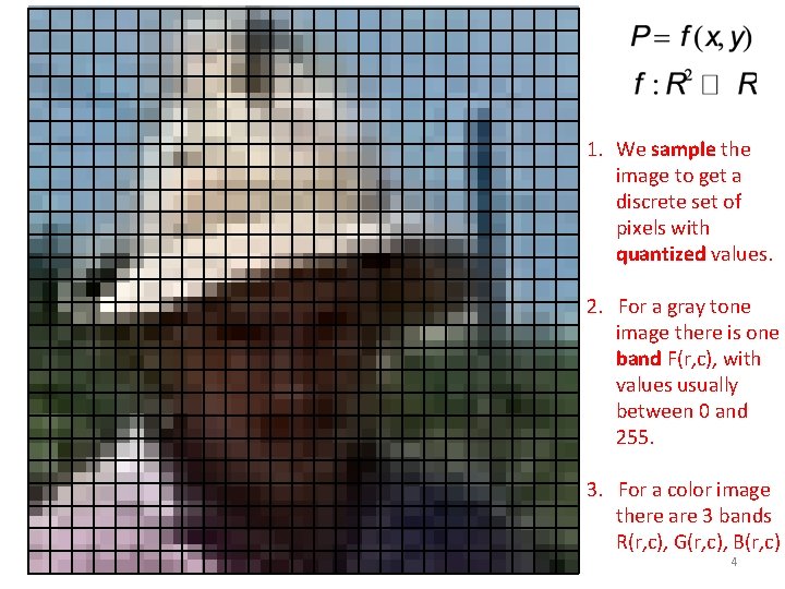
1. We sample the image to get a discrete set of pixels with quantized values. 2. For a gray tone image there is one band F(r, c), with values usually between 0 and 255. 3. For a color image there are 3 bands R(r, c), G(r, c), B(r, c) 4

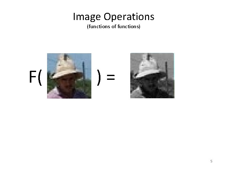
Image Operations (functions of functions) F( )= 5

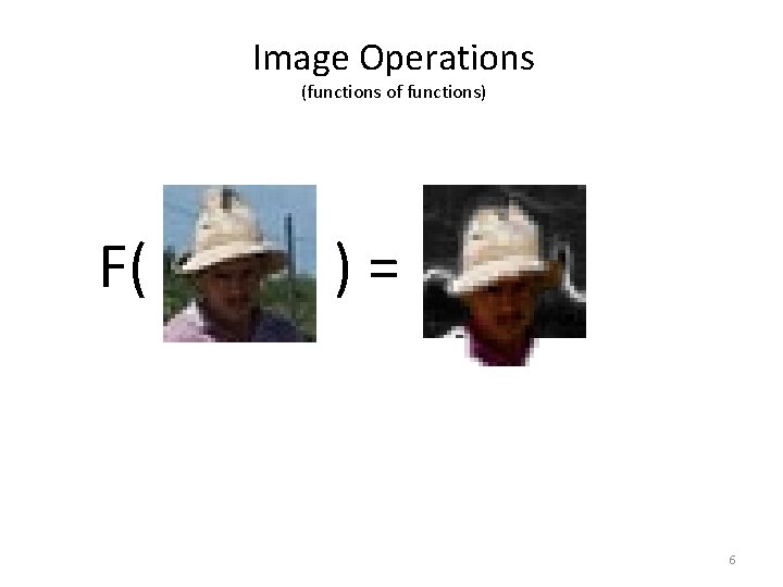
Image Operations (functions of functions) F( )= 6

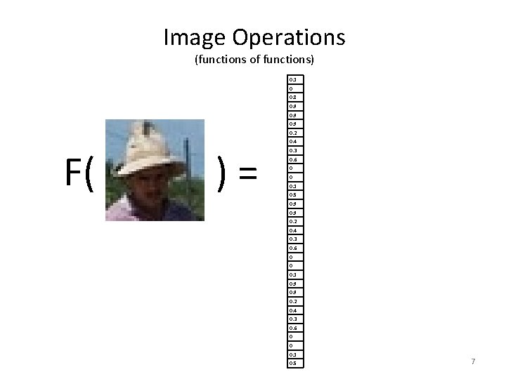
Image Operations (functions of functions) 0. 1 0 0. 8 0. 9 0. 2 F( )= 0. 4 0. 3 0. 6 0 0 0. 1 0. 5 0. 9 0. 2 0. 4 0. 3 0. 6 0 0 0. 1 0. 5 7

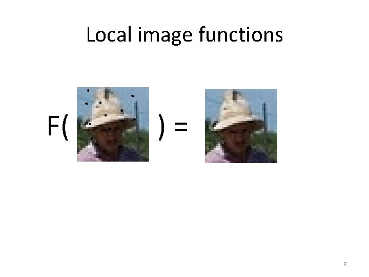
Local image functions F( )= 8

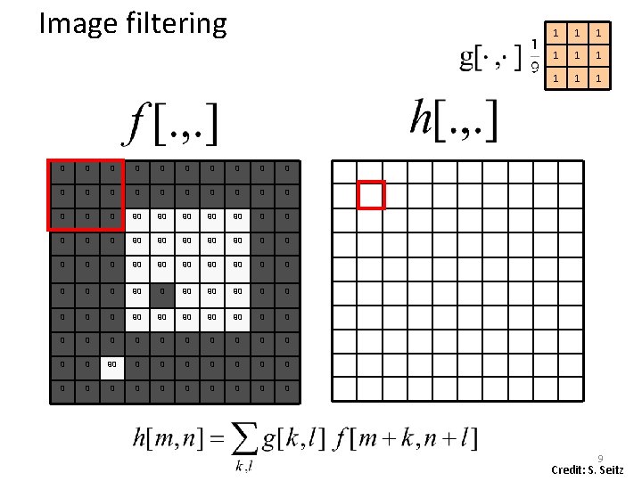
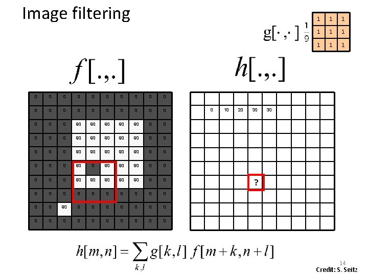
Image filtering 0 0 0 0 0 0 90 90 90 0 0 90 90 90 0 0 0 0 90 90 90 0 0 90 90 90 0 0 0 0 0 0 0 90 90 0 0 0 0 0 0 0 0 1 1 1 1 1 0 9 Credit: S. Seitz

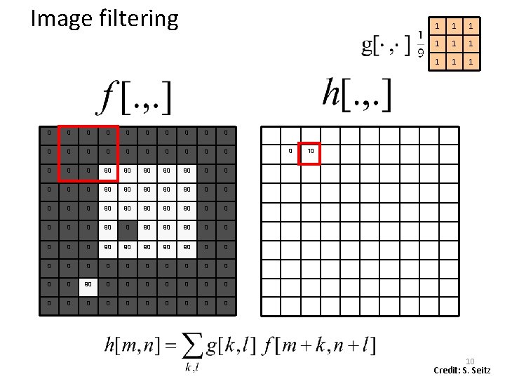
Image filtering 0 0 0 0 0 0 90 90 90 0 0 90 90 90 0 90 90 90 0 0 0 0 0 0 0 0 0 1 1 10 10 Credit: S. Seitz

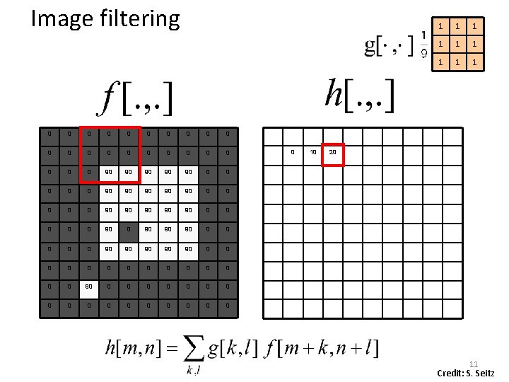
Image filtering 0 0 0 0 0 0 90 90 90 0 0 90 90 90 0 90 90 90 0 0 0 0 0 0 0 0 0 10 1 1 1 1 1 20 11 Credit: S. Seitz

Image filtering 0 0 0 0 0 0 90 90 90 0 0 90 90 90 0 90 90 90 0 0 0 0 0 0 0 0 0 10 20 1 1 1 1 1 30 12 Credit: S. Seitz

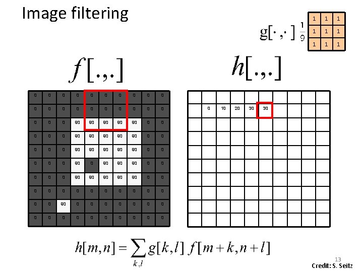
Image filtering 0 0 0 0 0 0 90 90 90 0 0 90 90 90 0 90 90 90 0 0 0 0 0 0 0 0 0 10 20 30 1 1 1 1 1 30 13 Credit: S. Seitz

Image filtering 0 0 0 0 0 0 90 90 90 0 0 90 90 90 0 90 90 90 0 0 0 0 0 0 0 0 0 10 20 30 1 1 1 1 1 30 ? 14 Credit: S. Seitz

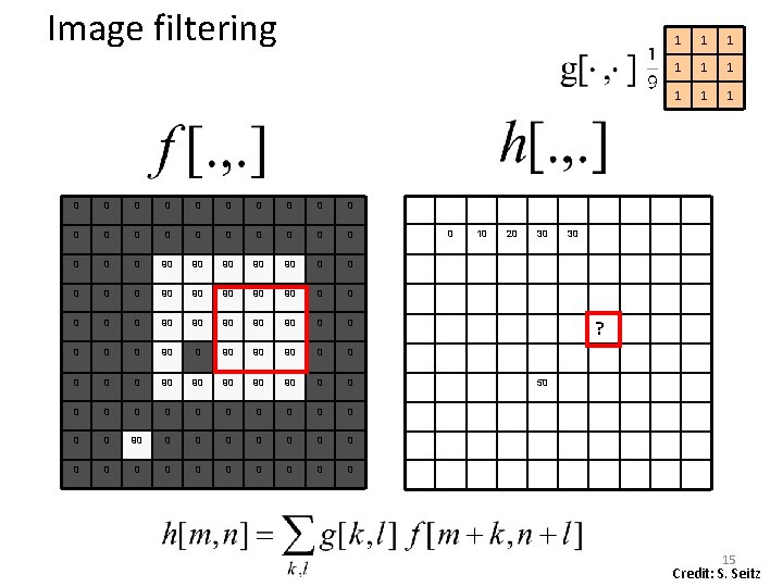
Image filtering 0 0 0 0 0 0 90 90 90 0 0 90 90 90 0 90 90 90 0 0 0 0 0 0 0 0 0 10 20 30 1 1 1 1 1 30 ? 50 15 Credit: S. Seitz

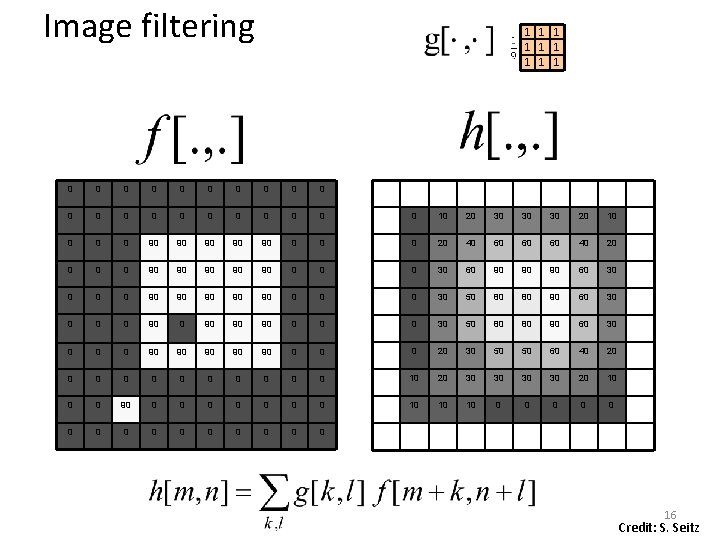
Image filtering 1 1 1 1 1 0 0 0 0 0 0 10 20 30 30 30 20 10 0 90 90 90 0 20 40 60 60 60 40 20 0 90 90 90 0 30 60 90 90 90 60 30 0 90 90 90 0 30 50 80 80 90 60 30 0 90 90 90 0 20 30 50 50 60 40 20 0 0 10 20 30 30 20 10 0 0 90 0 0 0 10 10 10 0 0 0 16 Credit: S. Seitz

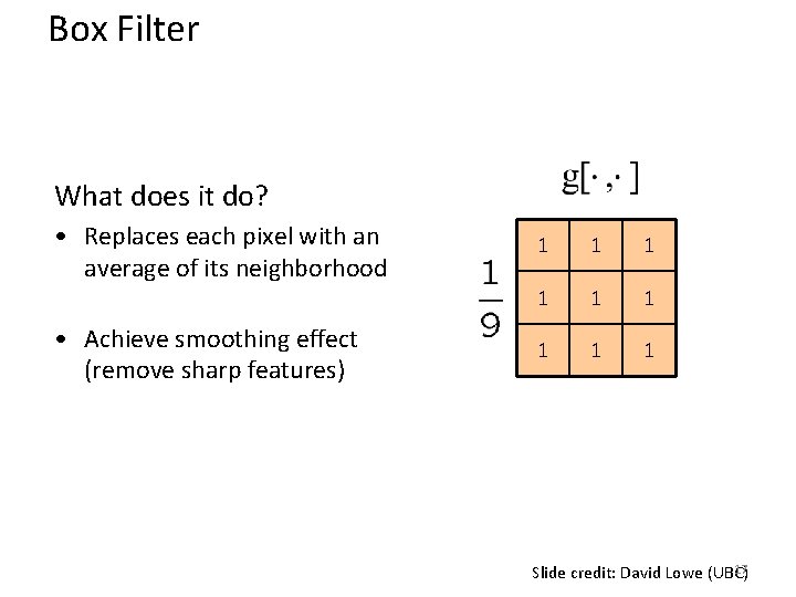
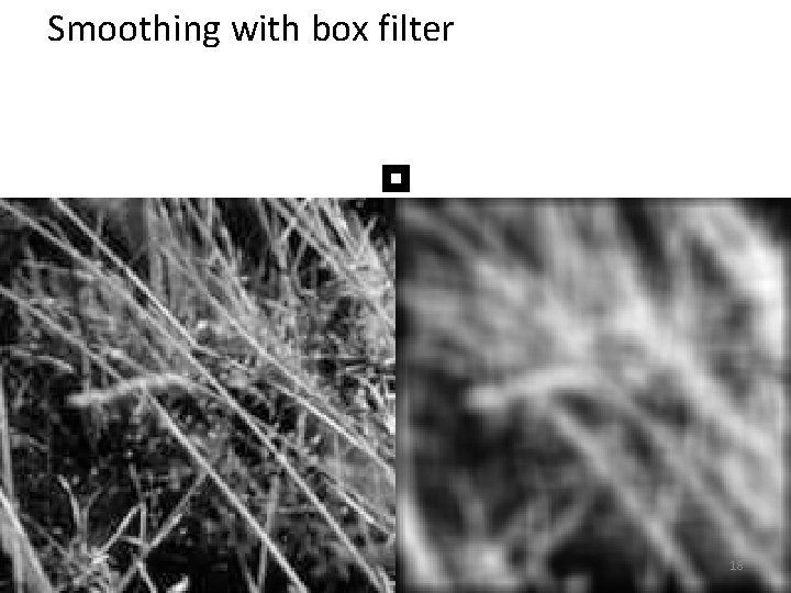
Box Filter What does it do? • Replaces each pixel with an average of its neighborhood • Achieve smoothing effect (remove sharp features) 1 1 1 1 17 Slide credit: David Lowe (UBC)

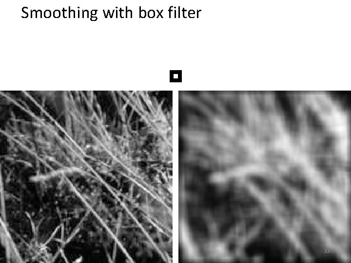
Smoothing with box filter 18

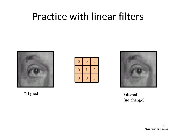
Practice with linear filters 0 0 1 0 0 ? Original 19 Source: D. Lowe

Practice with linear filters Original 0 0 1 0 0 Filtered (no change) 20 Source: D. Lowe

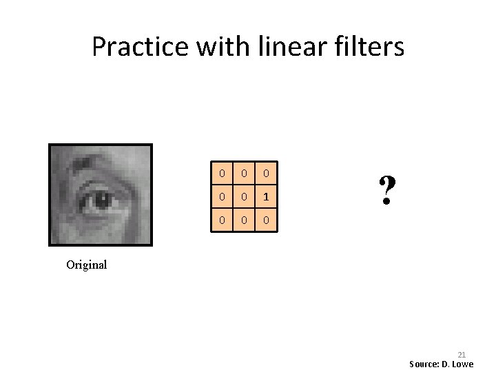
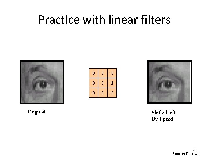
Practice with linear filters 0 0 0 1 0 0 0 ? Original 21 Source: D. Lowe

Practice with linear filters Original 0 0 0 1 0 0 0 Shifted left By 1 pixel 22 Source: D. Lowe

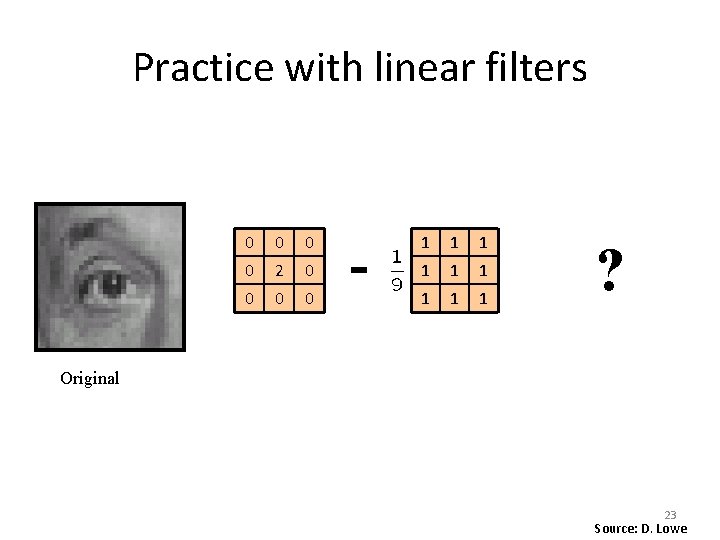
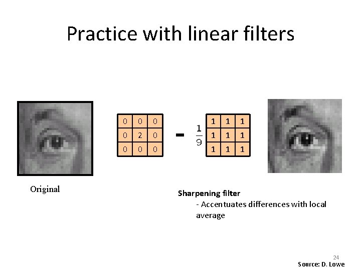
Practice with linear filters 0 0 2 0 0 - 1 1 1 1 1 ? Original 23 Source: D. Lowe

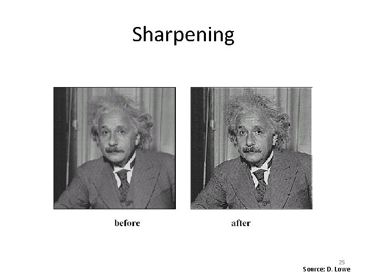
Practice with linear filters Original 0 0 2 0 0 - 1 1 1 1 1 Sharpening filter - Accentuates differences with local average 24 Source: D. Lowe

Sharpening 25 Source: D. Lowe

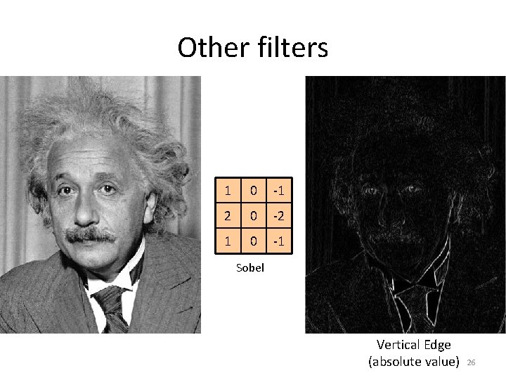
Other filters 1 0 -1 2 0 -2 1 0 -1 Sobel Vertical Edge (absolute value) 26

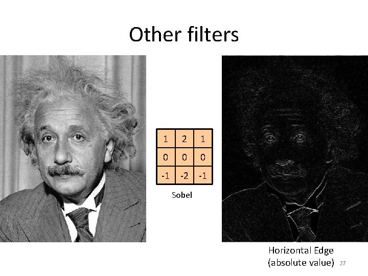
Other filters 1 2 1 0 0 0 -1 -2 -1 Sobel Horizontal Edge (absolute value) 27

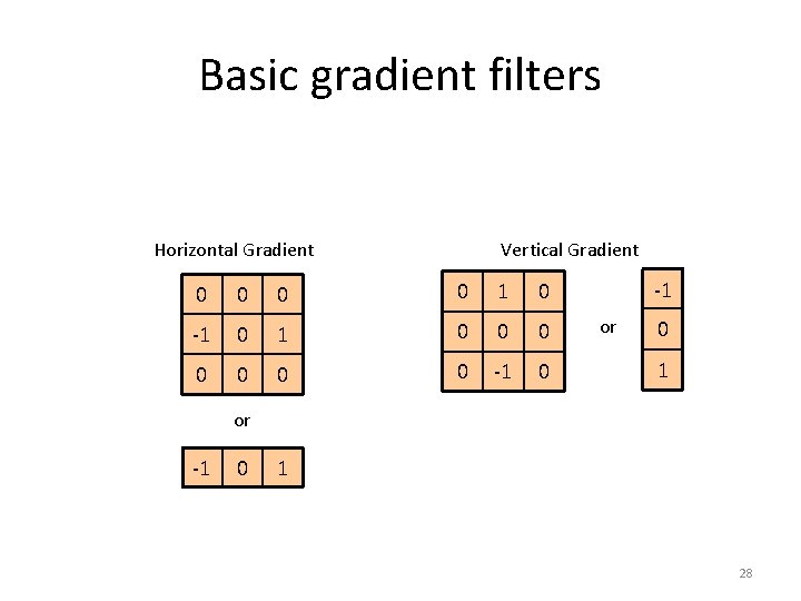
Basic gradient filters Horizontal Gradient Vertical Gradient 0 0 1 0 -1 0 0 0 0 -1 or 0 1 or -1 0 1 28

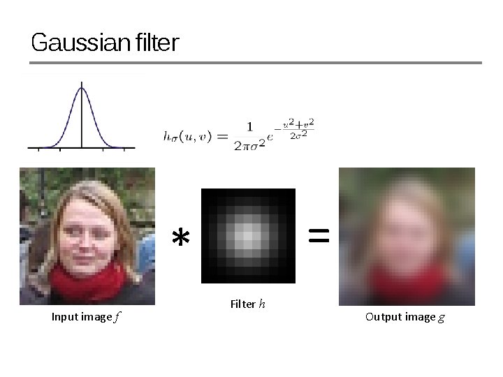
Gaussian filter = * Input image f Filter h Output image g

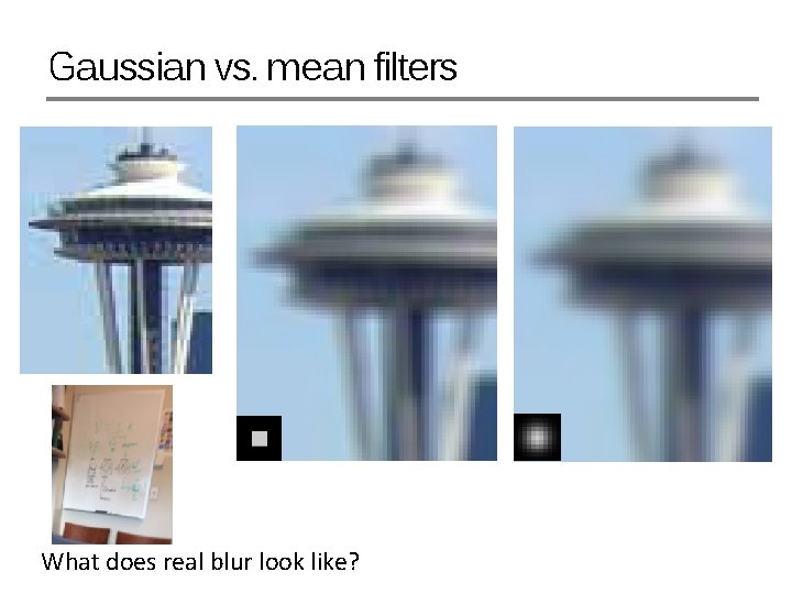
Gaussian vs. mean filters What does real blur look like?

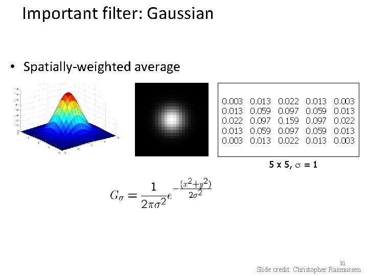
Important filter: Gaussian • Spatially-weighted average 0. 003 0. 013 0. 022 0. 013 0. 003 0. 013 0. 059 0. 097 0. 059 0. 013 0. 022 0. 097 0. 159 0. 097 0. 022 0. 013 0. 059 0. 097 0. 059 0. 013 0. 003 0. 013 0. 022 0. 013 0. 003 5 x 5, = 1 31 Slide credit: Christopher Rasmussen

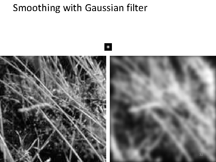
Smoothing with Gaussian filter 32

Smoothing with box filter 33

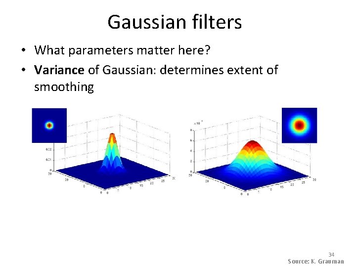
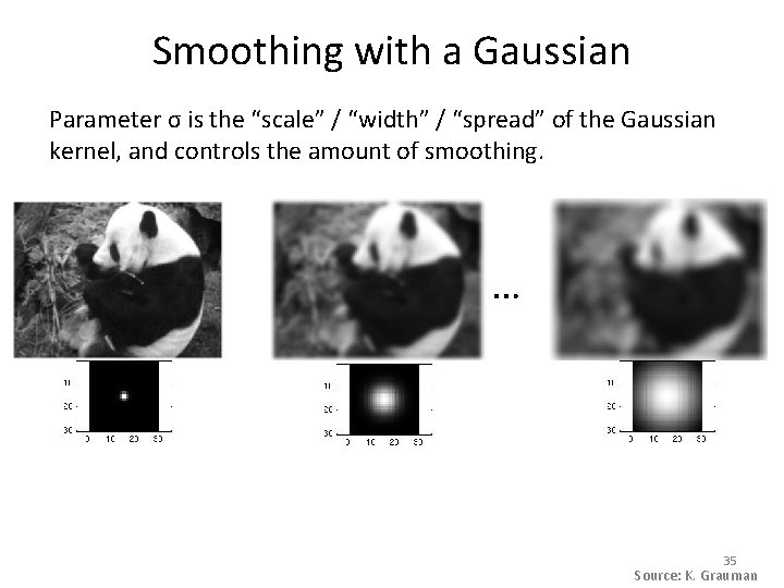
Gaussian filters • What parameters matter here? • Variance of Gaussian: determines extent of smoothing 34 Source: K. Grauman

Smoothing with a Gaussian Parameter σ is the “scale” / “width” / “spread” of the Gaussian kernel, and controls the amount of smoothing. … 35 Source: K. Grauman

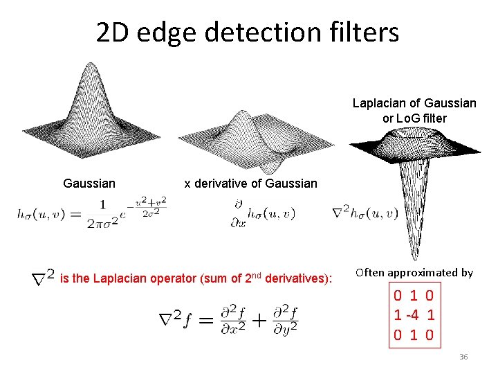
2 D edge detection filters Laplacian of Gaussian or Lo. G filter Gaussian x derivative of Gaussian is the Laplacian operator (sum of 2 nd derivatives): Often approximated by 0 1 -4 1 0 36

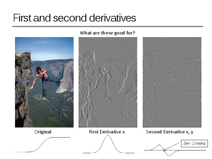
First and second derivatives What are these good for? Original First Derivative x Second Derivative x, y

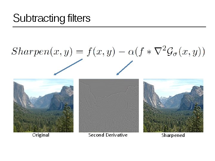
Subtracting filters Original Second Derivative Sharpened

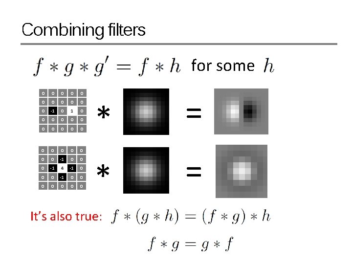
Combining filters for some 0 0 0 -1 0 0 0 0 0 -1 0 0 0 -1 4 -1 0 0 0 0 0 * = It’s also true:

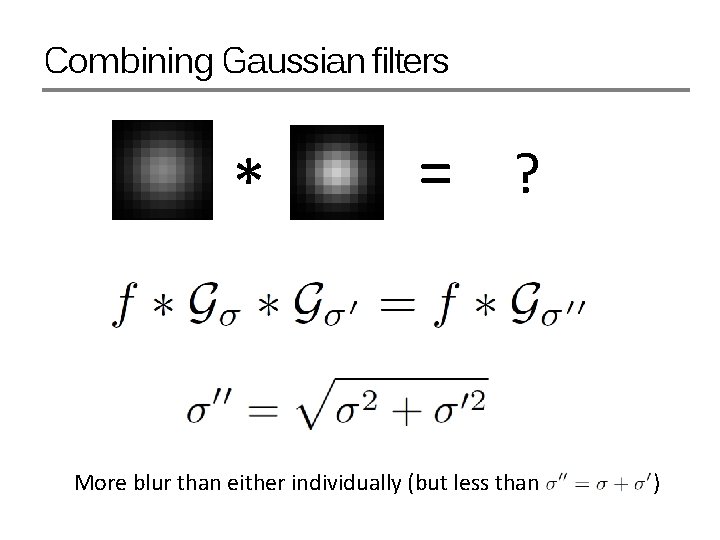
Combining Gaussian filters * = ? More blur than either individually (but less than )

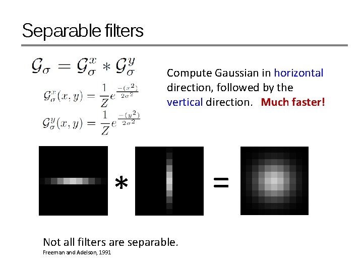
Separable filters Compute Gaussian in horizontal direction, followed by the vertical direction. Much faster! * Not all filters are separable. Freeman and Adelson, 1991 =

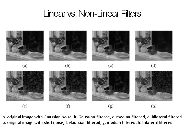
Linear vs. Non-Linear Filters a. original image with Gaussian noise, b. Gaussian filtered, c. median filtered, d. bilateral filtered e. original image with shot noise, f. Gaussian filtered, g. median filtered, h. bilateral filtered

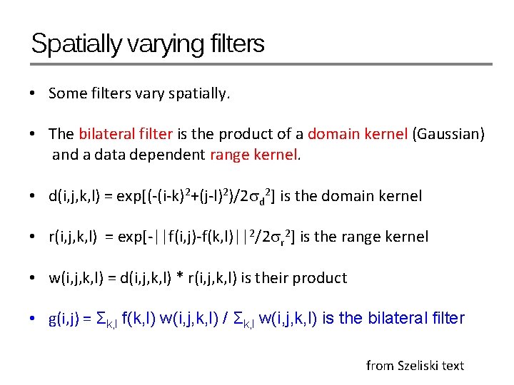
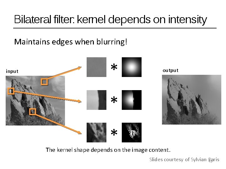
Spatially varying filters • Some filters vary spatially. • The bilateral filter is the product of a domain kernel (Gaussian) and a data dependent range kernel. • d(i, j, k, l) = exp[(-(i-k)2+(j-l)2)/2 d 2] is the domain kernel • r(i, j, k, l) = exp[-||f(i, j)-f(k, l)||2/2 r 2] is the range kernel • w(i, j, k, l) = d(i, j, k, l) * r(i, j, k, l) is their product • g(i, j) = Σk, l f(k, l) w(i, j, k, l) / Σk, l w(i, j, k, l) is the bilateral filter from Szeliski text

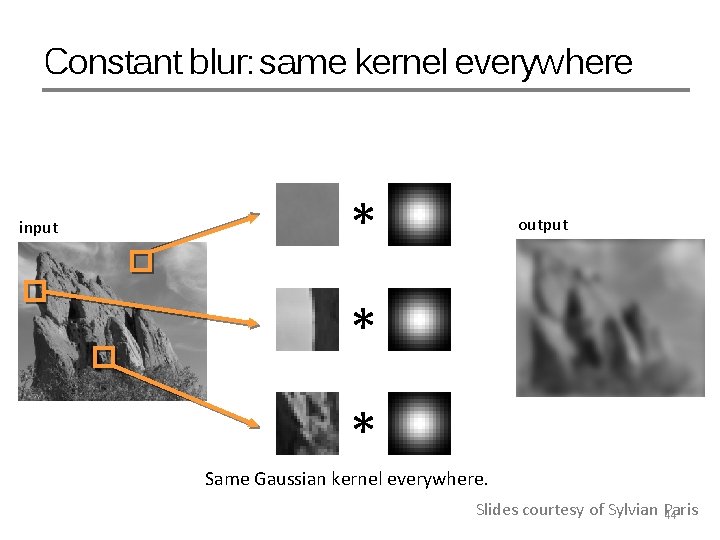
Constant blur: same kernel everywhere input * output * * Same Gaussian kernel everywhere. Slides courtesy of Sylvian Paris 44

Bilateral filter: kernel depends on intensity Maintains edges when blurring! input * output * * The kernel shape depends on the image content. Slides courtesy of Sylvian Paris 45

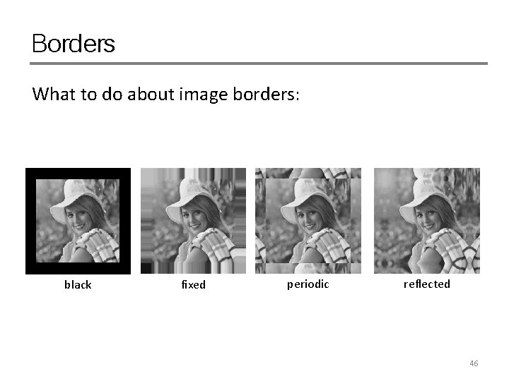
Borders What to do about image borders: black fixed periodic reflected 46

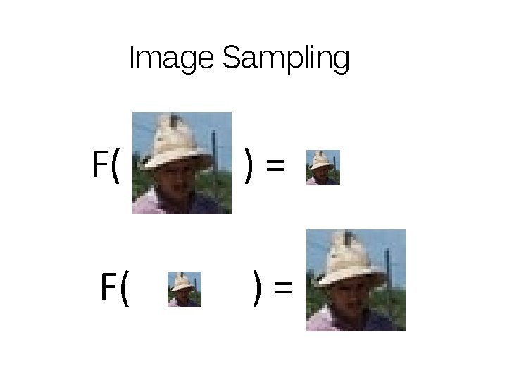
Image Sampling F( )=

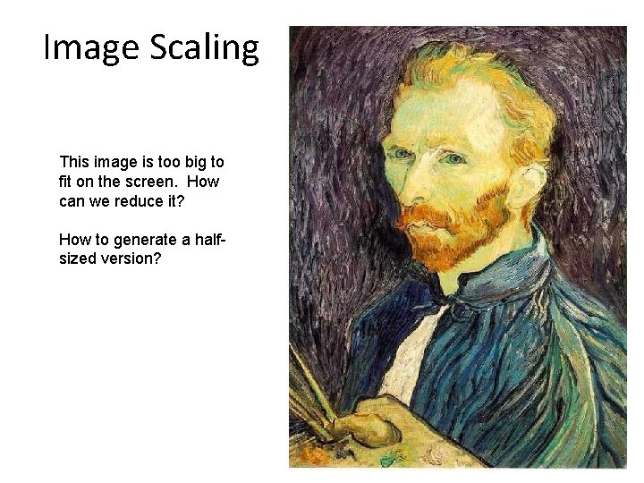
Image Scaling This image is too big to fit on the screen. How can we reduce it? How to generate a halfsized version?

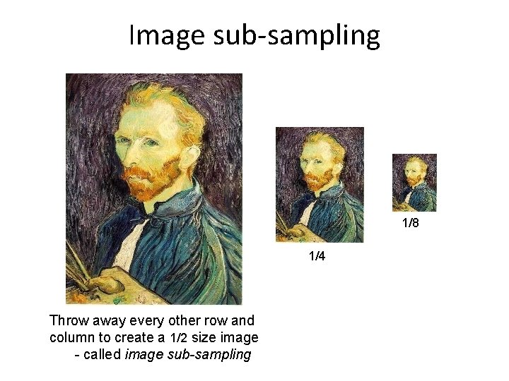
Image sub-sampling 1/8 1/4 Throw away every other row and column to create a 1/2 size image - called image sub-sampling

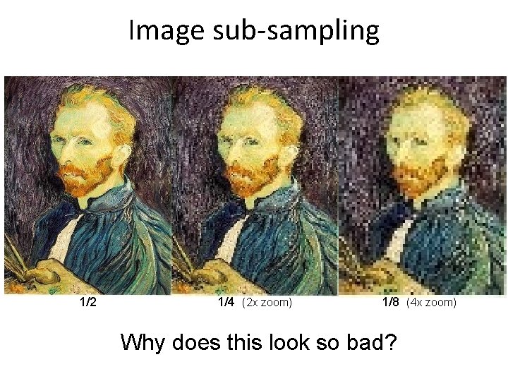
Image sub-sampling 1/2 1/4 (2 x zoom) 1/8 (4 x zoom) Why does this look so bad?

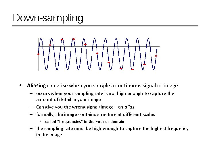
Down-sampling • Aliasing can arise when you sample a continuous signal or image – occurs when your sampling rate is not high enough to capture the amount of detail in your image – Can give you the wrong signal/image—an alias – formally, the image contains structure at different scales • called “frequencies” in the Fourier domain – the sampling rate must be high enough to capture the highest frequency in the image

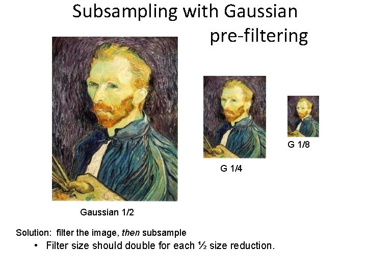
Subsampling with Gaussian pre-filtering G 1/8 G 1/4 Gaussian 1/2 Solution: filter the image, then subsample • Filter size should double for each ½ size reduction.

Finale • Filtering is just applying a mask to an image. • Computer vision people call the linear form of these operations “convolutions”. They are actually “correlations, ” since the true convolution inverts the mask. • There are many nonlinear filters, too, such as median filters and morphological filters. • Filtering is the lowest level of image analysis and is taught heavily in image processing courses. 53