FiducciaMattheyses FM algorithm Modified version of KL A

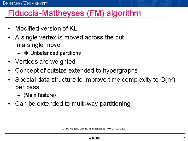
Fiduccia-Mattheyses (FM) algorithm • Modified version of KL • A single vertex is moved across the cut in a single move – Unbalanced partitions • Vertices are weighted • Concept of cutsize extended to hypergraphs • Special data structure to improve time complexity to O(n 2) per pass – (Main feature) • Can be extended to multi-way partitioning C. M. Fiduccia and R. M. Mattheyses, 19 th DAC, 1982. [Bazargan] 2

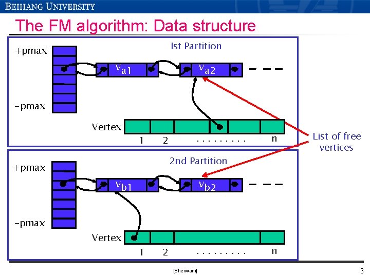
The FM algorithm: Data structure Ist Partition +pmax va 1 va 2 -pmax Vertex 1 2 . . n 2 nd Partition +pmax vb 1 List of free vertices vb 2 -pmax Vertex 1 2 . . [Sherwani] n 3

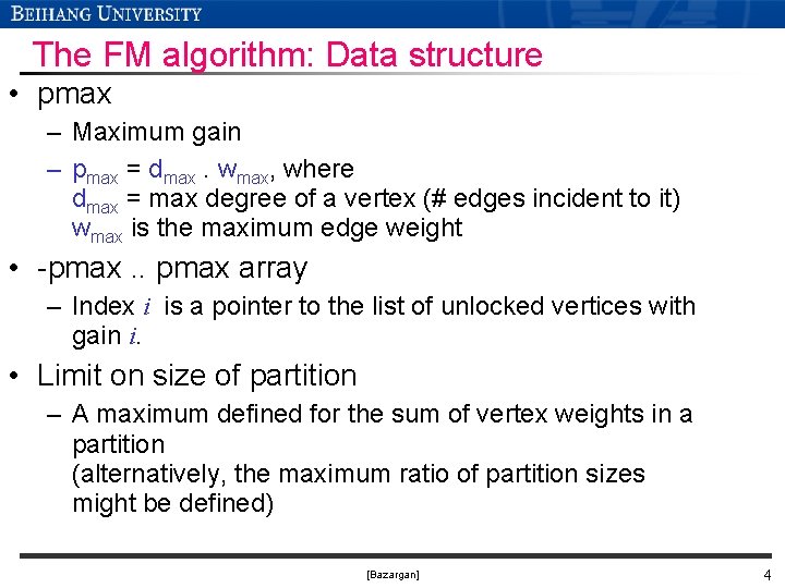
The FM algorithm: Data structure • pmax – Maximum gain – pmax = dmax. wmax, where dmax = max degree of a vertex (# edges incident to it) wmax is the maximum edge weight • -pmax. . pmax array – Index i is a pointer to the list of unlocked vertices with gain i. • Limit on size of partition – A maximum defined for the sum of vertex weights in a partition (alternatively, the maximum ratio of partition sizes might be defined) [Bazargan] 4

The FM algorithm • Initialize – Start with a balanced partition A, B of G (can be done by sorting vertex weights in decreasing order, placing them in A and B alternately) • Iterations – Similar to KL – A vertex cannot move if violates the balance condition – Choosing the node to move: pick the max gain in the partitions – Moves are tentative (similar to KL) – When no moves possible or no more unlocked vertices available, the pass ends – When no move can be made in a pass, the algorithm terminates [Bazargan] 5

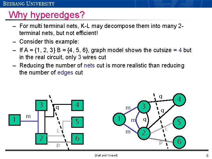
Why hyperedges? – For multi terminal nets, K-L may decompose them into many 2 terminal nets, but not efficient! – Consider this example: – If A = {1, 2, 3} B = {4, 5, 6}, graph model shows the cutsize = 4 but in the real circuit, only 3 wires cut – Reducing the number of nets cut is more realistic than reducing the number of edges cut 3 1 q m 2 k p q 4 5 3 m 1 m m 6 [Sait and Yousef] 4 q q 2 k p 5 6 6

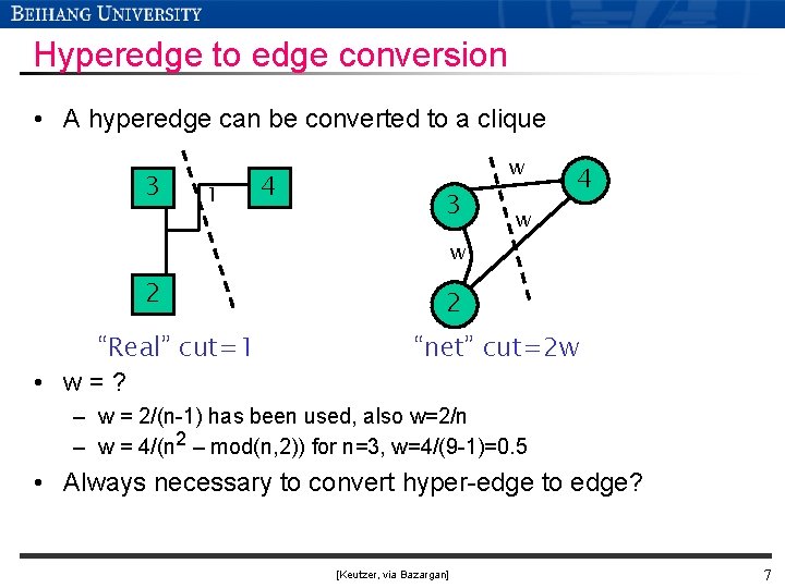
Hyperedge to edge conversion • A hyperedge can be converted to a clique 3 1 4 w 3 4 w w 2 “Real” cut=1 • w=? 2 “net” cut=2 w – w = 2/(n-1) has been used, also w=2/n – w = 4/(n 2 – mod(n, 2)) for n=3, w=4/(9 -1)=0. 5 • Always necessary to convert hyper-edge to edge? [Keutzer, via Bazargan] 7

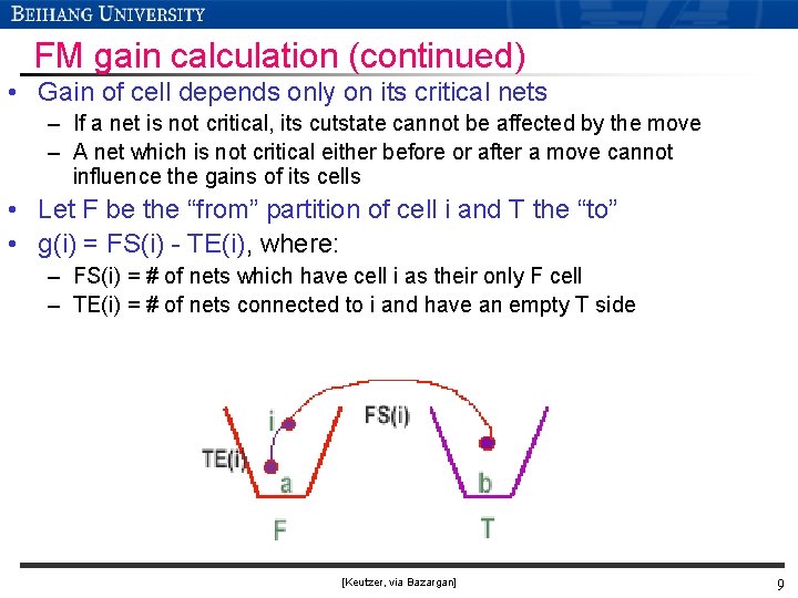
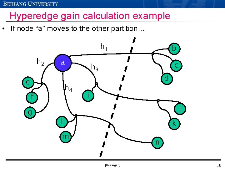
FM gain calculation: Direct hyperedge calc • FM is able to calculate gain directly using hyperedges ( not necessary to convert hyperedges to edges) • Definition: – Given a partition (A|B), we define the terminal distribution of n as an ordered pair of integers (A(n), B(n)), which represents the number of cells net n has in blocks A and B respectively (how fast can be computed? ) – Net is critical if there exists a cell on it such that if it were moved it would change the net’s cut state (whether it is cut or not). – Net is critical if A(n)=0, 1 or B(n)=0, 1 [Keutzer, via Bazargan] 8

FM gain calculation (continued) • Gain of cell depends only on its critical nets – If a net is not critical, its cutstate cannot be affected by the move – A net which is not critical either before or after a move cannot influence the gains of its cells • Let F be the “from” partition of cell i and T the “to” • g(i) = FS(i) - TE(i), where: – FS(i) = # of nets which have cell i as their only F cell – TE(i) = # of nets connected to i and have an empty T side [Keutzer, via Bazargan] 9

Hyperedge gain calculation example • If node “a” moves to the other partition… h 1 h 2 a e h 4 f g b c h 3 d i j l k m n [Bazargan] 10

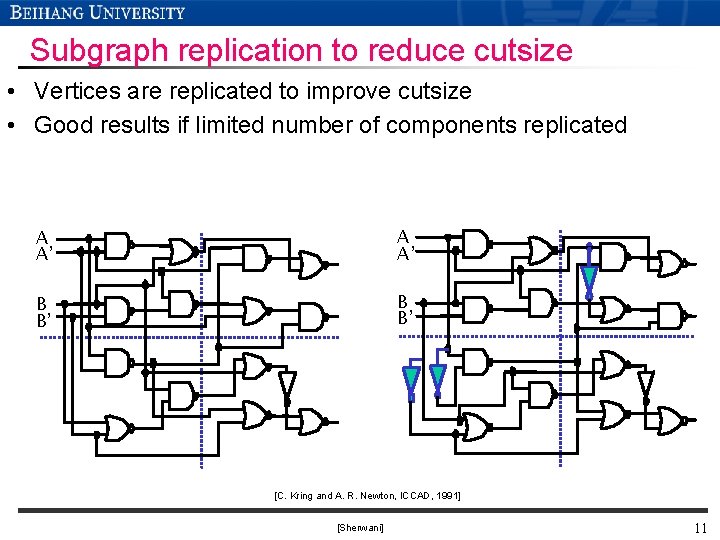
Subgraph replication to reduce cutsize • Vertices are replicated to improve cutsize • Good results if limited number of components replicated A A’ B B’ [C. Kring and A. R. Newton, ICCAD, 1991] [Sherwani] 11

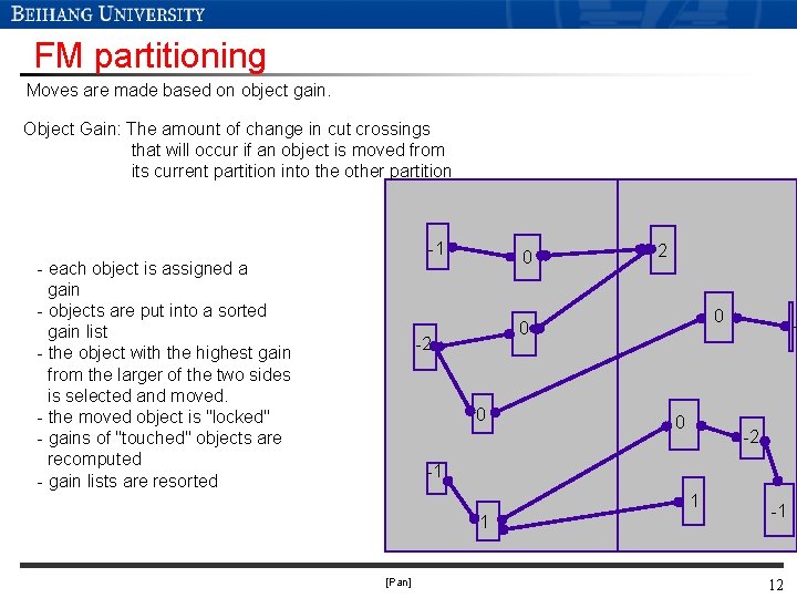
FM partitioning Moves are made based on object gain. Object Gain: The amount of change in cut crossings that will occur if an object is moved from its current partition into the other partition -1 - each object is assigned a gain - objects are put into a sorted gain list - the object with the highest gain from the larger of the two sides is selected and moved. - the moved object is "locked" - gains of "touched" objects are recomputed - gain lists are resorted 0 2 0 0 - -2 -1 1 1 [Pan] -1 12

FM partitioning -1 0 2 0 0 - -2 -1 1 1 [Pan] -1 13

FM partitioning -1 -2 -2 0 0 - -2 -1 1 1 [Pan] -1 14

FM partitioning -1 -2 -2 0 0 - -2 -1 1 [Pan] 1 -1 15

FM partitioning -1 -2 -2 0 -1 [Pan] 0 1 - -2 1 -1 16

FM partitioning -1 -2 -2 0 1 [Pan] -2 -1 -1 - -2 -1 17

FM partitioning -1 -2 -2 0 1 [Pan] - 0 -2 -1 -1 -2 -1 18

FM partitioning -1 -2 -2 -2 0 0 1 [Pan] -2 -1 -1 -2 -1 19

FM partitioning -1 -2 -2 0 -2 1 [Pan] -2 -1 -1 -2 -1 20

FM partitioning -1 -2 -2 0 -2 -2 1 -1 [Pan] -1 -2 -1 21

FM partitioning -1 -2 -2 0 -2 -2 1 -1 [Pan] -1 -2 -1 22

FM partitioning -1 -2 -2 0 -2 -1 -3 [Pan] -2 -1 23

FM partitioning -1 -2 -2 0 -1 -2 -2 -3 [Pan] -1 -2 -1 24

FM partitioning -1 -2 -2 0 -1 -2 -2 -3 [Pan] -1 -2 -1 25

FM partitioning -1 -2 -2 -3 [Pan] -1 -2 -1 26

Time complexity of FM • For each pass, – Constant time to find the best vertex to move. – After each move, time to update gain buckets is proportional to degree of vertex moved. – Total time is O(p), where p is total number of pins • Number of passes is usually small. [Pan] 27

Extensions

Tie-breaking strategy • For each vertex, instead of having a gain bucket, a gain vector is used. • Gain vector is a sequence of potential gain values corresponding to numbers of possible moves into the future. • Therefore, rth entry looks r moves ahead. • Time complexity is O(pr), where r is max # of look-ahead moves stored in gain vector. • If ties still occur, some researchers observe that LIFO order improves solution quality. “An Improved Min-Cut Algorithm for Partitioning VLSI Networks”, IEEE Trans. Computers, 33(5): 438 -446, 1984. [Pan] 29

Ratio cut objective • It is not desirable to have some pre-defined ratio on the partition sizes. • Wei and Cheng proposed the Ratio Cut objective. • Try to locate natural clusters in circuit and force the partitions to be of similar sizes at the same time. • Ratio Cut RXY = CXY/(|X| x |Y|) • A heuristic based on FM was proposed. “Towards Efficient Hierarchical Designs by Ratio Cut Partitioning”, ICCAD, pages 1: 298 -301, 1989. [Pan] 30

Multi-way partitioning • Dividing into more than 2 partitions. • Algorithm by extending the idea of FM + Krishnamurthy. L. Sanchis, “Multiple-way Network Partitioning, IEEE Trans. Computers, 38(1): 62 -81, 1989. [Pan] 31

Simulated annealing

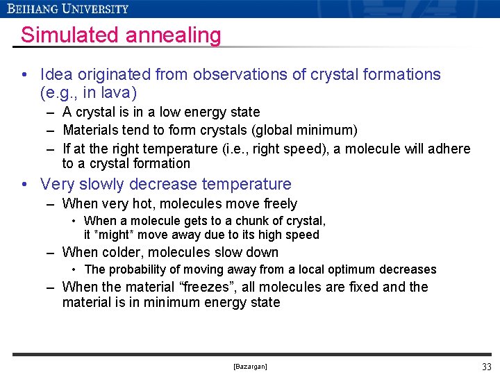
Simulated annealing • Idea originated from observations of crystal formations (e. g. , in lava) – A crystal is in a low energy state – Materials tend to form crystals (global minimum) – If at the right temperature (i. e. , right speed), a molecule will adhere to a crystal formation • Very slowly decrease temperature – When very hot, molecules move freely • When a molecule gets to a chunk of crystal, it *might* move away due to its high speed – When colder, molecules slow down • The probability of moving away from a local optimum decreases – When the material “freezes”, all molecules are fixed and the material is in minimum energy state [Bazargan] 33

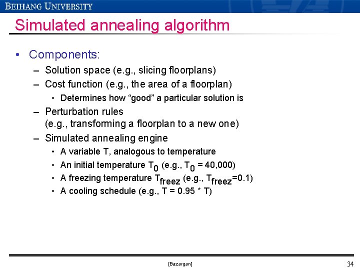
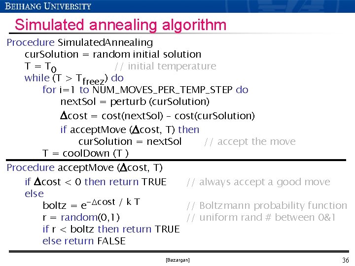
Simulated annealing algorithm • Components: – Solution space (e. g. , slicing floorplans) – Cost function (e. g. , the area of a floorplan) • Determines how “good” a particular solution is – Perturbation rules (e. g. , transforming a floorplan to a new one) – Simulated annealing engine • • A variable T, analogous to temperature An initial temperature T 0 (e. g. , T 0 = 40, 000) A freezing temperature Tfreez (e. g. , Tfreez=0. 1) A cooling schedule (e. g. , T = 0. 95 * T) [Bazargan] 34

Simulated annealing: More insight. . . Annealing steps [Bazargan] 35

Simulated annealing algorithm Procedure Simulated. Annealing cur. Solution = random initial solution T = T 0 // initial temperature while (T > Tfreez) do for i=1 to NUM_MOVES_PER_TEMP_STEP do next. Sol = perturb (cur. Solution) Dcost = cost(next. Sol) – cost(cur. Solution) if accept. Move (Dcost, T) then cur. Solution = next. Sol // accept the move T = cool. Down (T ) Procedure accept. Move (Dcost, T) if Dcost < 0 then return TRUE // always accept a good move else boltz = e-Dcost / k T // Boltzmann probability function r = random(0, 1) // uniform rand # between 0&1 if r < boltz then return TRUE else return FALSE [Bazargan] 36

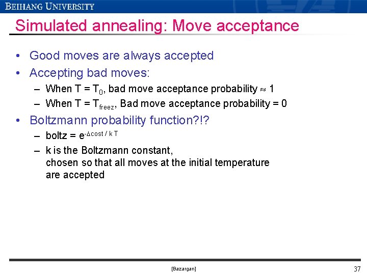
Simulated annealing: Move acceptance • Good moves are always accepted • Accepting bad moves: – When T = T 0, bad move acceptance probability 1 – When T = Tfreez, Bad move acceptance probability = 0 • Boltzmann probability function? !? – boltz = e-Dcost / k T – k is the Boltzmann constant, chosen so that all moves at the initial temperature accepted [Bazargan] 37

Simulated annealing: More insight. . . [Bazargan] 38

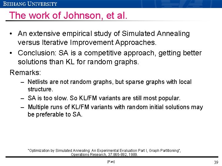
The work of Johnson, et al. • An extensive empirical study of Simulated Annealing versus Iterative Improvement Approaches. • Conclusion: SA is a competitive approach, getting better solutions than KL for random graphs. Remarks: – Netlists are not random graphs, but sparse graphs with local structure. – SA is too slow. So KL/FM variants are still most popular. – Multiple runs of KL/FM variants with random initial solutions may be preferable to SA. “Optimization by Simulated Annealing: An Experimental Evaluation Part I, Graph Partitioning”, Operations Research, 37: 865 -892, 1989. [Pan] 39

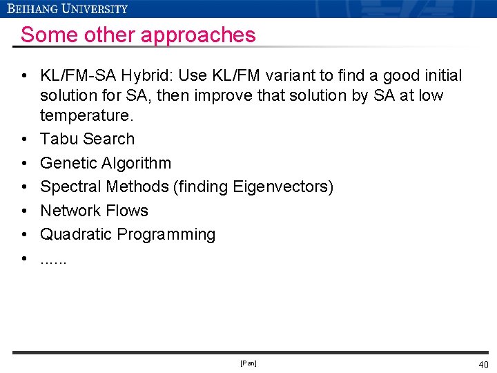
Some other approaches • KL/FM-SA Hybrid: Use KL/FM variant to find a good initial solution for SA, then improve that solution by SA at low temperature. • Tabu Search • Genetic Algorithm • Spectral Methods (finding Eigenvectors) • Network Flows • Quadratic Programming • . . . [Pan] 40

• https: //web. archive. org/web/20081003192033/http: //www. s tanford. edu/~dgleich/demos/matlab/spectral. html 41

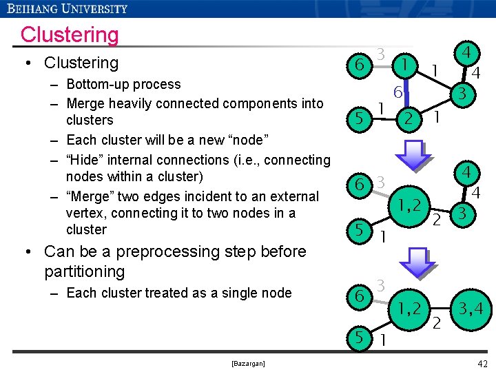
Clustering • Clustering – Bottom-up process – Merge heavily connected components into clusters – Each cluster will be a new “node” – “Hide” internal connections (i. e. , connecting nodes within a cluster) – “Merge” two edges incident to an external vertex, connecting it to two nodes in a cluster • Can be a preprocessing step before partitioning – Each cluster treated as a single node 6 5 3 1 6 2 1 1 4 6 3 4 1, 2 2 3 5 1 6 3 5 1 [Bazargan] 1 4 4 3 1, 2 2 3, 4 42

Multilevel hypergraph partitioning

Multi-level partitioning G. Karypis, R. Aggarwal, V. Kumar and S. Shekhar, DAC 1997. [Pan] 44

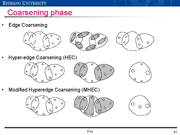
Coarsening phase • Edge Coarsening • Hyper-edge Coarsening (HEC) • Modified Hyperedge Coarsening (MHEC) [Pan] 45

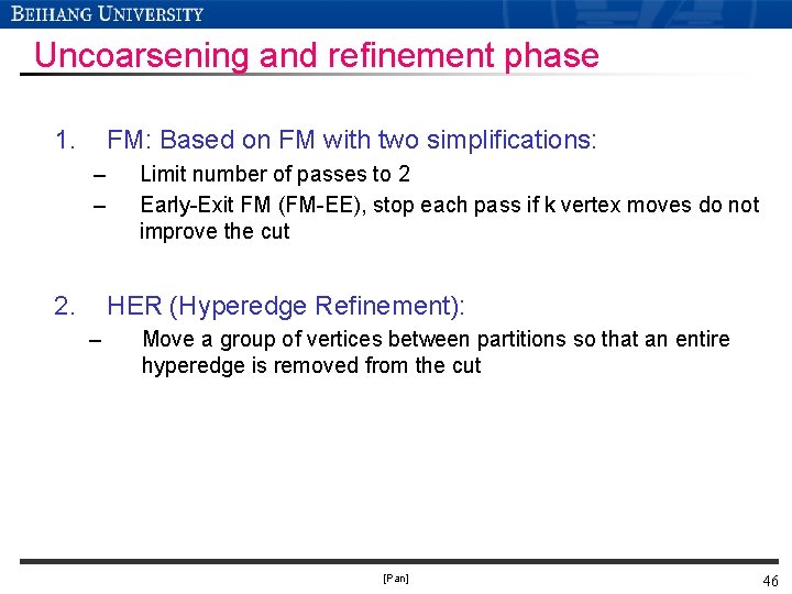
Uncoarsening and refinement phase 1. FM: Based on FM with two simplifications: – – 2. Limit number of passes to 2 Early-Exit FM (FM-EE), stop each pass if k vertex moves do not improve the cut HER (Hyperedge Refinement): – Move a group of vertices between partitions so that an entire hyperedge is removed from the cut [Pan] 46

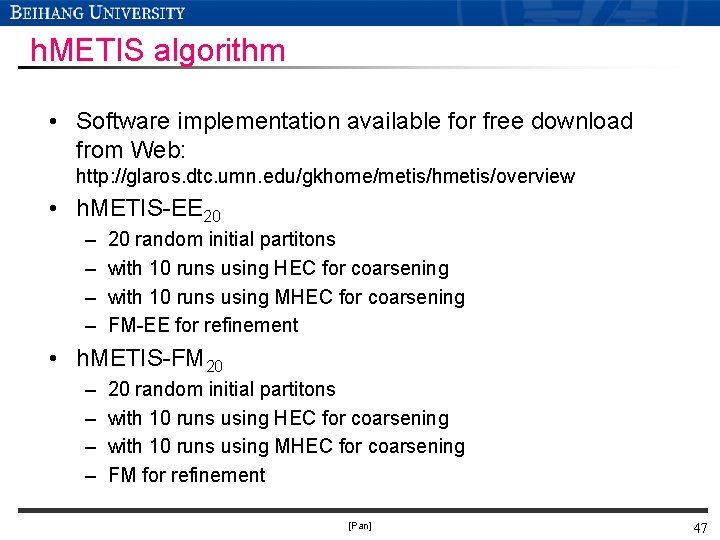
h. METIS algorithm • Software implementation available for free download from Web: http: //glaros. dtc. umn. edu/gkhome/metis/hmetis/overview • h. METIS-EE 20 – – 20 random initial partitons with 10 runs using HEC for coarsening with 10 runs using MHEC for coarsening FM-EE for refinement • h. METIS-FM 20 – – 20 random initial partitons with 10 runs using HEC for coarsening with 10 runs using MHEC for coarsening FM for refinement [Pan] 47

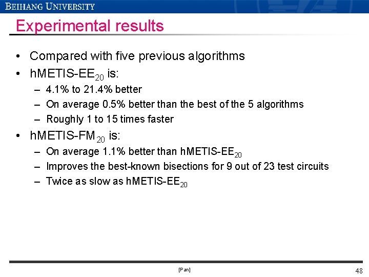
Experimental results • Compared with five previous algorithms • h. METIS-EE 20 is: – 4. 1% to 21. 4% better – On average 0. 5% better than the best of the 5 algorithms – Roughly 1 to 15 times faster • h. METIS-FM 20 is: – On average 1. 1% better than h. METIS-EE 20 – Improves the best-known bisections for 9 out of 23 test circuits – Twice as slow as h. METIS-EE 20 [Pan] 48