Estimation of population parameters Confidence intervals A Normal

Estimation of population parameters (Confidence intervals)

A) Normal d. B) Non-normal d. Population (parameters): , Sample (statistics): x, s x Calculation of confidence intervals allows us to express the precision of the estimate of true parameters.

A) Normal Distribution 1) Confidence Interval for the Mean: 2) Limits: L 1 (lower), L 2 (upper) L 1 x Standard error of the mean: L 2 Population ( ) (SEM, SE) Samp. 1 Samp. 2 Samp. 3 = measure of the precision with which a sample mean true population mean . estimates the

• If the sample size increases -> SEM decreases (precision with which we estimate the true mean increases) • If sample is more variable (SD increases) -> SEM increases (precision with which we estimate the true mean decreases) (True mean value of population will lie within the interval AVG SEM)

We can determine a specific precision of the calculation by error = 0. 05 or 0. 01 (used for biological data) ( different spreads of the interval: 95% or 99% confidence level) t , – confidence coefficient (=critical value from tables of t-distribution) - dependent on chosen and =n-1)

Confidence coefficient = critical value (is determined by and error )

Calculation of confidence intervals for the mean: Example: Body weights (in kg) of 25 piglets: xi : 25. 8, 24. 6, 26. 1, 22. 9, 25. 1, 27. 3, 24. 0, 24. 5, 23. 9, 26. 2, 24. 3, 24. 6, 23. 3, 25. 5, 28. 1, 24. 8, 23. 5, 26. 3, 25. 4, 25. 5, 23. 9, 27. 0, 24. 8, 22. 9, 25. 4. Mean: SEM: At the 95% confidence level: =24 t(0. 05, 24)= 2. 064 At the 99% confidence level: =24 t(0. 01, 24)= 2. 797

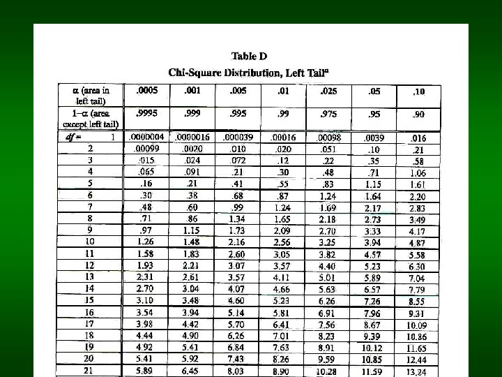
A) Normal Distribution 2) Confidence interval for the SD ( ): 21 - /2 , 2 /2 – confident coefficients (tables of chi-square distribution)

f( f( 2) 2 /2 21 - /2 2 2 /2 – left tail value upper limit of the interval 21 - /2 – right tail value lower limit of the interval

B) Non-normal Distribution 1) Confidence interval for the median: 2) Limits L 1, L 2 = values derived from the statistical tables : according to n and we find out ranks for L 1, L 2. We replace these ranks with the actual values from the variant sequence.

Confidence Interval for the Median = 0. 05 n 8 9 10 11 12 13 14. . . 100 (Part of table) Lower Limit Upper Limit 1 2 2 2 3 3 3. . . 40 8 8 9 10 10 11 12. . . 61 Confidence interval: L 1=13. 5 L 2=16. 8 Sample (n=14) x 1 x 2 x 3 x 4 x 5 x 6. . . x 12 x 13 x 14 12. 3 12. 8 13. 5 14. 1 14. 3 14. 9. . . 16. 8 17. 0 17. 1

Statistical Hypotheses Testing (Research data evaluation)

The major goal of statistical analysis is to draw conclusions regarding a population by examining a sample from that population. We start by creating a Hypothesis = a statement regarding a population characteristics: its distribution or parameters (mean, SD). For example: Population matches Gaussian normal distribution 2 populations have the same mean 2 populations have the same variance

This hypothesis is called a null hypothesis (H 0) – it expresses the concept of „no difference“. For example: H 0 : = const. (e. g. the population mean is equal to 25. 3 kg) 1 = 2 (2 populations have the same mean) 12 = 22 (2 populations have the same variance) If it is concluded that a null hypothesis is false, then an alternate hypothesis (HA) is assumed to be true. HA denies H 0 : const. 1 2 1 2 2 2

The use in practice: experimental data evaluation. E. g. : we need to find out if a vitamin supplement in food causes an increase of body weight in piglets. Experiment: group 1 of piglets (Test sample) gets the vitamin supplement in food group 2 of piglets (Control sample) gets standard food After some period we measure the body weight in both samples: Test Control

We have to decide, whether the difference between sample means is only random (caused by variability of animals) – or whether it is big enough to conclude, that the difference was caused by experimental activity. It would mean that this experimental activity is generally effective (population means would be different as well). In this case we can reject the null hypothesis: 1 = 2. Conclusion: Hypothesis: „the increase of body weight is caused by vitamin supplement“ is generally true (increase of body weight is not random).

Decision rule about an acceptance of the hypothesis = Statistical Test. The statistical test consists of Test Statistic calculation: E. g. : t – testing for difference between 2 means (t-test) F– testing for difference between 2 variances (F-test) 2 – testing for difference between 2 frequencies ( 2 -test)

Types of Statistical Tests Parametric – testing for difference between sets that follow the normal distribution – hypotheses concerning and are tested Nonparametric – for sets following the nonnormal distribution – hypotheses concerning common characteristics of statistical sets are tested (e. g. two sets have the same shape of distribution)

Parametric Tests (Normal Distribution: Hypotheses concerning and )

F-test (Variance Ratio Test) If we have two samples, each taken at random from a normal population, we might ask if the variances of 2 populations are equal. Test for differences between 2 variances: (H 0: 12= 22) Sample 1: n 1, s 12 Sample 2: n 2, s 22 Test statistic:

F–test – Conclusion: If calculated F > Fcrit. 12 22 (significant difference between variances: variability of 2 populations is not equal) If calculated F Fcrit. 12= 22 (insignificant difference between variances: variability of 2 populations is equal)

F-test – Use: Ø we are concern in the effect of experiment affecting the variability of studied biological character Ø before t-test (test for differences between 2 means)

Example: By means of F-test we have to decide, whether duck clutch size is differently variable in captive than in wild birds. Clutch Size of Ducks (number of eggs): Captive Wild 10 11 12 11 10 11 11 DF = 6 n 1=7 s 12= 0. 48 9 8 11 12 10 13 11 10 12 n 2=9 DF = 8 s 22= 2. 50 F 0. 05= 4. 15 (crit. value) DF =n-1 F >F 0. 05 we reject H 0: 12= 22 Clutch sizes in captive and in wild ducks are differently variable. (P<0. 05)

a - chosen error of statistical calculations Biological data: most often 5%