Environmental and Exploration Geophysics I Terrain Conductivity tom

Environmental and Exploration Geophysics I Terrain Conductivity tom. h. wilson tom. wilson@geo. wvu. edu Phone - 293 -6431 Department of Geology and Geography West Virginia University Morgantown, WV Tom Wilson, Department of Geology and Geography

Calculating measured terrain conductivity Main objective for the day is to develop an understanding of the computational approach discussed in the text on pages 514 -518. For more detail see Mc. Neill’s technical note on EM Conductivity at Low Induction Number • Basic definitions • Units conversions [ohm/m <>mmhos/m] • Relative and cumulative response functions • The representation of subsurface geology translated into the relative response function • Calculating terrain conductivity - a • Two and 3 layer problems • Problem assignments

Additional scope for the day’s activities • Discuss computational procedures used to compute a. • We will introduce ideas presented in Mc. Neill’s Technical Note to provide broader context and background on the computational approach. • Relative and cumulative response functions will be introduced. • Class problems will be limited to vertical dipole computations outlined by Berger et al. • We’ll go into much more detail than Berger with the objective of giving you some understanding of the underlying basis for the computation. • In class problem

Basic ideas to re-familiarize yourself with … • Coulomb law (inverse square relationship) • Lorentz relation (force on a charge moving through a region containing both an electric and magnetic fields. • Basic vector notions associated with interactions between a moving charge and ambient magnetic field. • Right hand rule • Magnetic field lines associated with a bar magnet and current flowing through a coil • Faraday’s law of induction • Lenz’s law • Ohm’s law *Visit basic ideas link under lecture topic 3 of class web page.

Basic definitions V is potential difference Ohm’s Law i current R resistance Resistance, defined as opposition to direct current flow, is not a fundamental physical attribute of materials since it varies depending on the conductor geometry. The geometrical influences are evident in this relationship where is the resistivity, l the conductor length, and A the cross-sectional area of the conductor

A or l The resistivity represents a fundamental physical property of the conductor, and this or its inverse (the conductivity) are the parameters we wish to measure. In general - Resistivity is the property of a material which resists current flow.

Units The unit of resistance is the ohm Balancing units in the definitional formula for resistivity, we see that resistivity has units of ohm-meters or -m. Conductance is the reciprocal of resistance and has units of ohm-1. Thus conductivity ( ) has units of ohm-1/m or mho/meter

Working back and forth between units of conductivity and resistivity • The reciprocal of a resistivity of 1 -m corresponds to a conductivity of 1 mho/meter • 1 mho/meter = 1000 millimhos/meter • 1 millimho/meter =0. 001 mho/meters • The reciprocal of 0. 001 mho/meters is 1000 -m Conductance (1/R) is often measured in units of Seimens (S) which are equivalent to mhos. 1 S = 1 mho

Tom Wilson, Department of Geology and Geography

In general when given a resistance the equivalent conductivity in millimhos/meter is obtained by taking the inverse of the resistivity and multiplying by 1000. The same applies to the computation of resistivity when given the conductivity. Consider the following … 100 -m = _____ millimhos/meter 20 millimhos/meter = _____ -m

Text Errors 1) The function R is incorrectly referred to as the relative response function; it is the cumulative response function. 2) There is an error in the math (e. g. page 517, equation 8. 32). Basically you cannot incorporate the instrument height into the solution the way they do. We will always assume that instrument is on the ground. So make a note …. Z should not include instrument height above the ground! Assume that the coils are on the ground surface. Z= (depth)/(intercoil spacing) Any equation they use that includes depth plus 1 meter (instrument height) is incorrect. Tom Wilson, Department of Geology and Geography

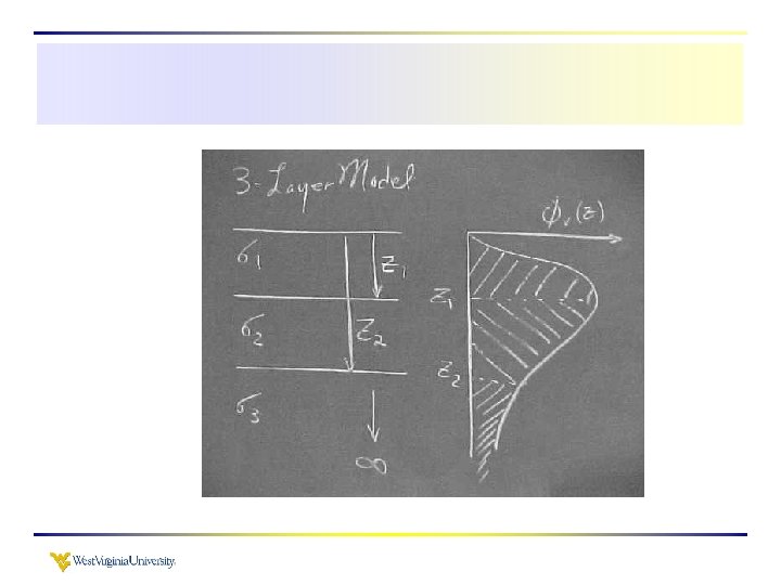
For most of today’s lecture we are going to discuss the computation of a for simple models of the type shown below. This example comes from Mc. Neil’s Technical Note that Z= depth/intercoil spacing

Relative response functions (i. e. Mc. Neill) Note that the relative response function for the horizontal dipole h is much more sensitive to near-surface conductivity variations and that its response or sensitivity drops off rapidly with depth Vertical dipole interaction has no sensitivity to surface conductivity, reaches peak sensitivity at z ~0. 5, and is more sensitive to conductivity at greater depths than is the horizontal dipole.

Example presented by Mc. Neill

Constant conductivity The contribution of this thin layer to the overall ground conductivity is proportional to the value of the relative response function at that depth.

Z 1 Z 2 The contribution of a layer to the overall ground conductivity is proportional to the area under the relative response function over the range of depths (Z 2 -Z 1) spanned by that layer.

As you might expect, the contribution to ground conductivity of a layer of constant conductivity that extends significant distances beneath the surface (i. e. homogenous half-space) is proportional to the total area under the relative response function.

So in general the contribution of several layers to the overall ground conductivity will be in proportion to the areas under the relative response function spanned by each layer.

You all will recognize these area diagrams as integrals. The contribution of a given layer to the overall ground conductivity at the surface above it is proportional to the integral of the relative response function over the range of depths spanned by the layer.

Mc. Neill introduces another function, R(z) - the cumulative response function - which he uses to compute the ground conductivity from a given distribution of conductivity layers beneath the surface. For next time continue your reading of Mc. Neill and develop a general appreciation of the relative and cumulative response functions.

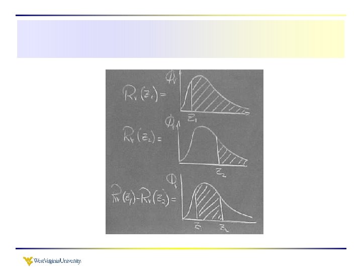
The following diagrams are intended to help you visualize the relationship between R(z) and (z). Each point on the RV(z) curve represents the area under the V(z) curve from z to .

Z 2

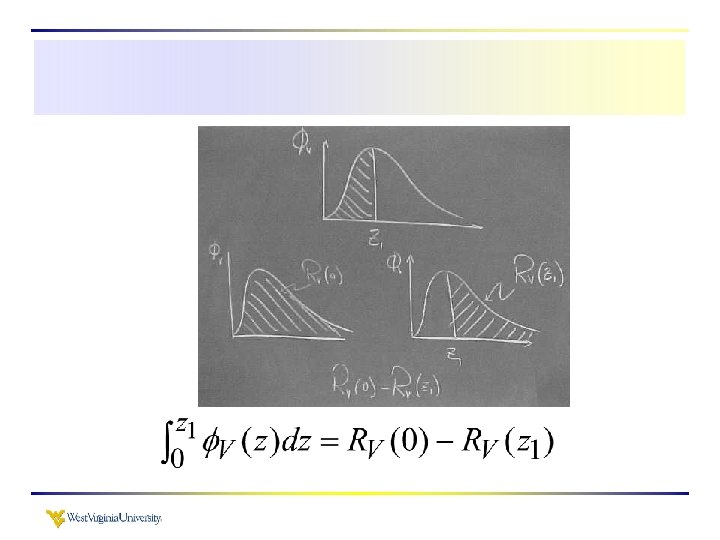
Consider one additional integral - How would you express this integral as a difference of cumulative response functions?

Note that R(0) = 1, hence

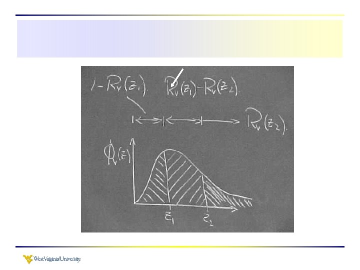
According to our earlier reasoning - the contribution of a single conductivity layer to the measured ground (or terrain) conductivity is proportional to the area under the relative response function. The apparent conductivity measured by the terrain conductivity meter at the surface is the sum total of the contributions from all layers. We know that each of the areas under the relative response curve can be expressed as a difference between cumulative response functions.

Let’s consider the following problem, which is taken directly from Mc. Neill’s technical report (TN 6).

Visually, the solution looks like this. .

Mathematical formulation - Compare this result to that of Mc. Neill’s (see page 8 TN 6).

In this relationship a is the apparent conductivity measured by the conductivity meter. The dependence of the apparent conductivity on intercoil spacing is imbedded in the values of z. Z for a 10 meter intercoil spacing will be different from z for the 20 meter intercoil spacing. The above equation is written in general form and applies to either the horizontal or vertical dipole configuration.

In the appendix of Mc. Neill (today’s handout), he notes that the assumption of low induction number yields simple algebraic expressions for the relative and cumulative response functions. We can use these relationships to compute specific values of R for given zs.

The simple algebraic expressions for RV(z) and RH(z) make it easy for us to compute the terms in the problem Mc. Neill gives us. In that problem z 1 is given as 0. 5 and z 2 as 1 and 1. 5 Assuming a vertical dipole orientation RV(z=0. 5) ~ 0. 71 RV(z=1. 0) ~ 0. 45 RV(z=1. 5) ~ 0. 32

1=20 mmhos/m Z 1 = 0. 5 2=2 mmhos/m Z 2 = 1 and 1. 5 3=20 mmhos/m Substituting in the following for the case where Z 2=1.

Problems 8. 5, 8. 6, and 8. 7 and AMD problem will be due next Tuesday Bring questions for discussion in class on this Thursday. Remember that papers on the Terrain Conductivity reading list are available in the 3 rd floor mail room.

Here’s a problem for you to work through before our next class. Mine spoil surface AMD contamination zone ~60 ft Pit Floor ~10 ft A terrain conductivity survey is planned using the EM 31 meter (3. 66 m (or 12 foot) intercoil spacing). Our hypothetical survey was conducted over a mine spoil to locate migration pathways within the spoil through which acidic mine drainage as well as neutralizing treatment are being transported. Scattered borehole data across the spoil suggest that these paths are approximately 10 feet thick and several meters in width. Borehole resistivity logs indicate that areas of the spoil surrounding these conduits have low conductivity averaging about 4 mmhos/m. The bedrock or pavement at the base of the spoil also has a conductivity of approximately 4 mmhos/m. Depth to the pavement in the area of the proposed survey is approximately 60 feet. Conductivity of the AMD transport channels is estimated to be approximately 100 mmhos/m.

Z. 000. 200. 400. 600. 800 1. 000 1. 200 1. 400 1. 600 1. 800 2. 000 2. 200 2. 400 2. 600 2. 800 3. 000 3. 200 3. 400 3. 600 3. 800 4. 000 4. 200 4. 400 4. 600 4. 800 5. 000 5. 200 5. 400 5. 600 5. 800 RV 1. 000000. 9284767. 7808688. 6401844. 5299989. 4472136. 3846154. 3363364. 2982750. 2676438. 2425356. 2216211. 2039542. 1888474. 1757906. 1643990. 1543768. 1454940. 1375683. 1304545. 1240347. 1182129. 1129097. 1080592. 1036061. 0995037. 0957124. 0921982. 0889320. 0858884 RH 1. 000000. 6770329. 4806249. 3620499. 2867962. 2360680. 2000000. 1732137. 1526108. 1363084. 1231055. 1122055. 1030602. 0952811. 0885849. 0827627. 0776539. 0731363. 0691128. 0655074. 0622578. 0593147. 0566359. 0541887. 0519428. 0498762. 0479660. 0461979. 0445547. 0430231