Environmental and Exploration Geophysics I Resistivity III tom

Environmental and Exploration Geophysics I Resistivity III tom. h. wilson tom. wilson@mail. wvu. edu Department of Geology and Geography West Virginia University Morgantown, WV

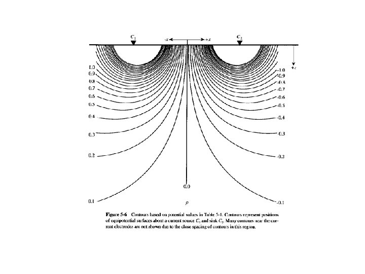
General ideas about potential field and current distributions.

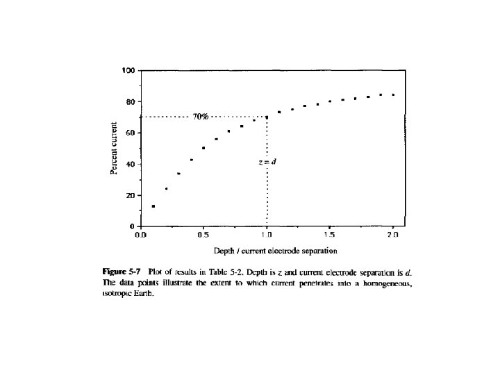
From the text we are given z is depth and d is electrode spacing

Current Fraction Wenner Array depth/a In the preceding diagram z was depth. In this diagram z is depth divided by a which is 1/3 rd the current electrode separation. Remember the a-spacing refers to the electrode spacing in the Wenner Array.

Change in potential - source to potential electrode Note the similarity of this “sensitivity” curve to the relative response function ( V(z)) used with terrain conductivity data. You can also think of this curve as indicating the contribution of intervals at various depths to the potential between one current and one potential electrode.

multiples of a We see that in general for the Wenner array the peak sensitivity of the array to subsurface resistivity distributions occurs at depths approximately equal to the a-spacing.

By comparison to the characterization of instrument response as a function of depth and intercoil spacing for the terrain conductivity method, the resistivity relationships are defined much more qualitatively. Mostly we have general rules of thumb.

Qualitative interpretation of a resistivity sounding - How many layers have been sensed in this resistivity sounding? The observations consist of apparent resistivities recorded at various a-spacings (Wenner array) or l-spacings (Schlumberger array). See empirical methods on pages 95 and 296 of Berger.

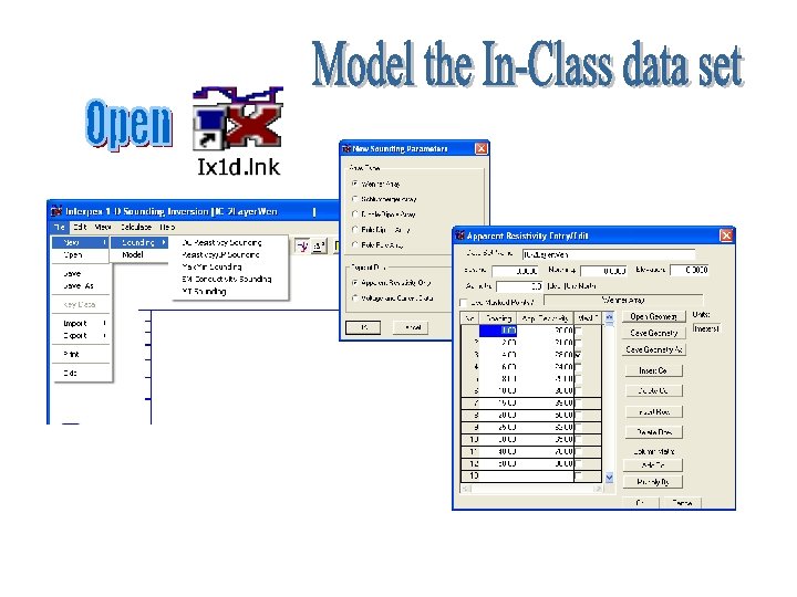
Let’s examine the utility of the interpolation approach using the in-class data set you worked up last week. Recall how to determine apparent resistivity?

The apparent resistivities ( a) are computed from the relationship we derived earlier. Where G = 2 a for the Wenner array

Here are some plots of our synthetic or “test” data set. The model from which it is derived is shown at lower right.

The Inflection Point Depth Estimation Procedure This technique suggests that the depths to various boundaries are related to inflection points in the apparent resistivity measurements. Again, the In-Class data set illustrates the utility of this approach. Apparent resistivities plotted below are shown over the model for both the Schlumberger and Wenner arrays. The inflection points are located, and dropped to the spacing-axis. The technique is suggested too be most applicable for use with the Schlumberger array. The inflection point rule varies with array type. For the Wenner array, the approximate depth to the interface is 1/2 the inflection point spacing. For the Schlumberger array this would give a depth to the top of the layer of about 12 meters instead of the actual depth of 8. In the case of the Wenner array we would get a depth of about 9 meters. A general “rule of thumb” for the Schlumberger array would to divide the inflection point distance by 3 instead of 2; that would yield 8 meters.

Resistivity determination through extrapolation This technique suggests that the actual resistivity of a layer can be estimated by extrapolating the trend of apparent resistivity variations toward some asymptote, as shown in the figure below. The problem with this is being able to correctly guess where the plateau or asymptote actually is. Spacings in the In-Class data set only go out to 50 meters. The model data set (below) used for the inflection point discussion reveals that this asymptote is reached only gradually, in this case at distances of 500 meters and greater. Since most of the layers affecting the apparent resistivity in our surveys will be associated with thin layers, we are unlikely to be able to do this very accurately. The apparent resistivity will vary considerably over that distance rather than rise gradually to resistivities of individual layers. At best the technique offers only a crude estimate.

Equivalence - non-uniqueness. . .

The realm of possibility. . .

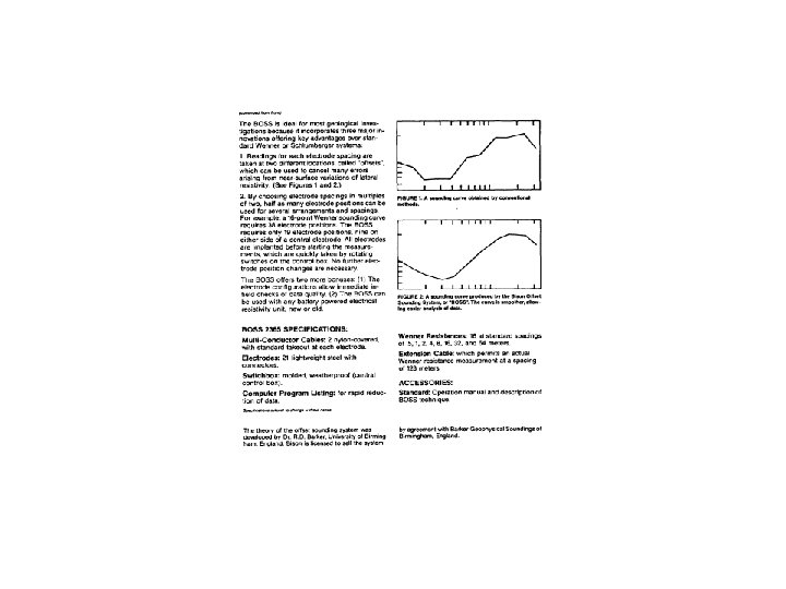
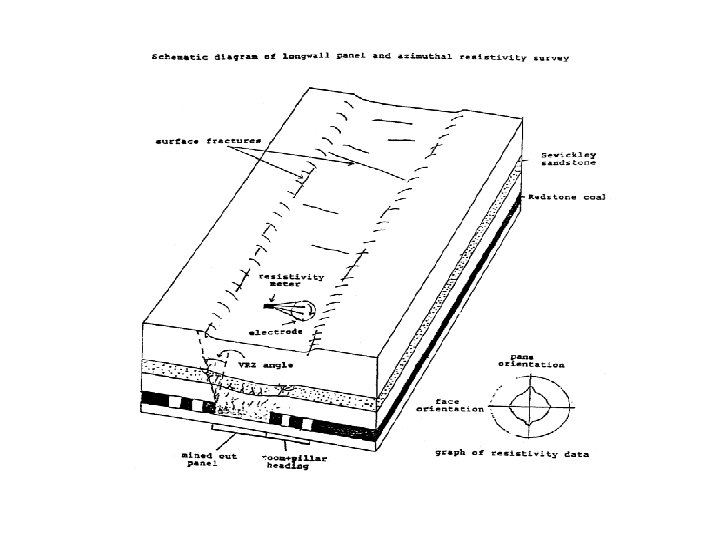
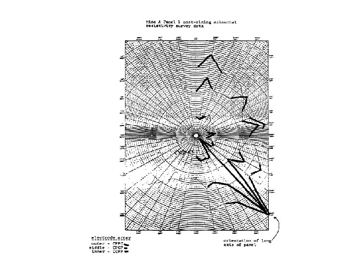
Multi-electrode resistivity systems

Tri-potential resistivity method

Normal Wenner array configuration

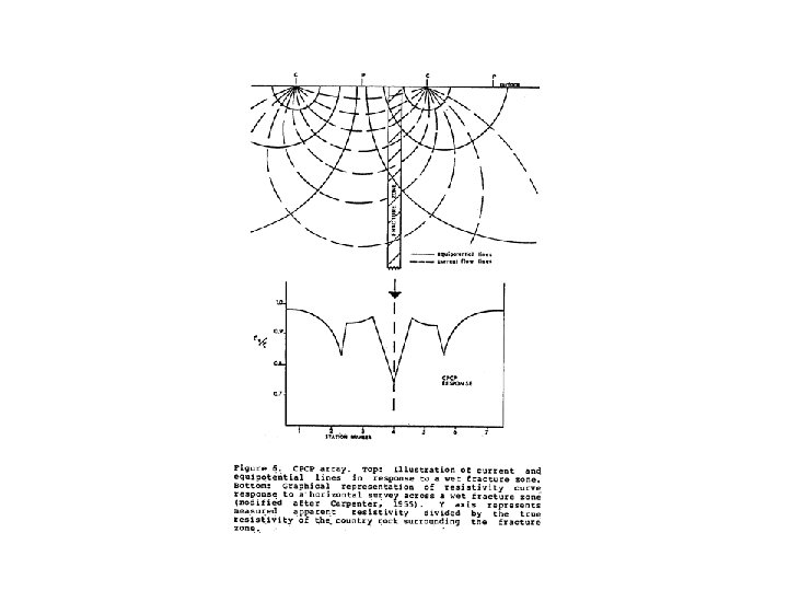
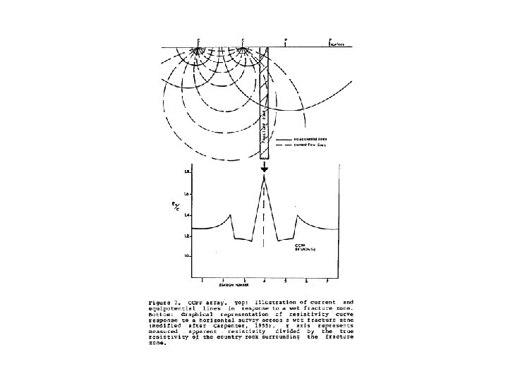
CCPP

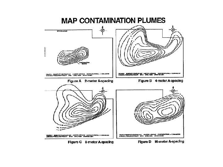
Some background information about the resistivity lab

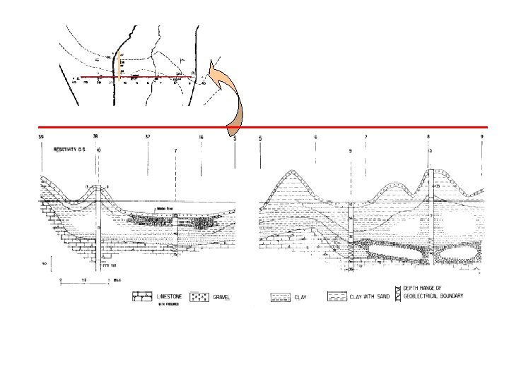
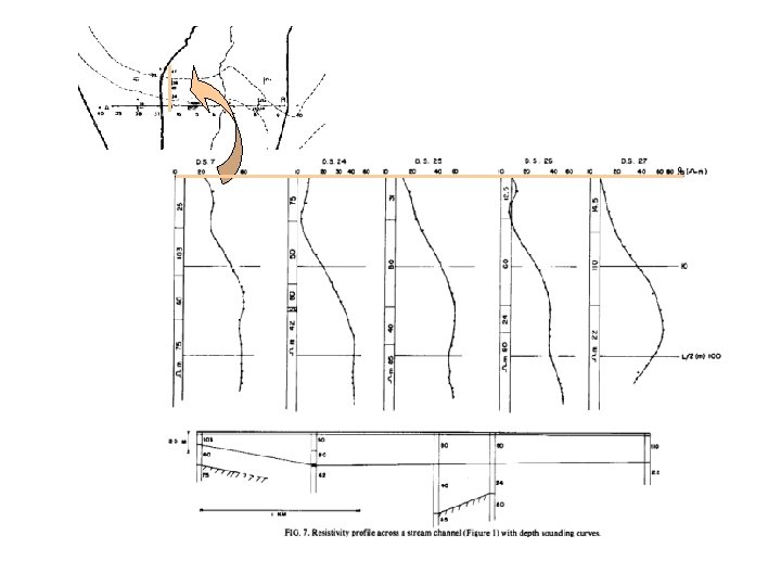
How well did Frohlich do? Let’s put his models to the test. a SS 5 depth

For class this Thursday test the resistivity model derived by Frohlich to explain the apparent resistivity variations observed in Sounding SS 3 (his D. S. 25) 1. Hand in a list of resistivities & depths you determined from the sounding shown at left. 2. Hand in a plot showing the comparison of apparent resistivities computed using his model and the apparent resistivities observed in the survey. 3. Comment on how well they match (what % error did you get? ) 4. Invert to obtain a better match using the same number of layers. 5. In a paragraph describe how your results differ from those obtained by Frohlich.

Next Class • Hand today’s assignment in on Thursday. • Lab is not due till the 11 th, but keep working on it. • There is a test next Thursday