ENT 356 Instrumentation System Lecture 3 Error Analysis

ENT 356 Instrumentation System Lecture 3 – Error Analysis Sem 2, 2010/2011 1

School of Mechatronics Engineering Error Analysis Introduction: In both science and engineering, we have theoretical & experimental studies……………… The way these two branches handle numerical data are significantly different… Your Car Is Traveling At 160 km/h…IS IT? ? Your Measured Body Weight Is 70 kg…. IS IT? ?

School of Mechatronics Engineering Error Analysis Introduction: For an honest die with an honest roll, each of the six faces are equally likely to be facing up after the throw. For a pair of dice, then, there are 6 × 6 = 36 equally likely combinations. Of these 36 combinations there is only one, 1 -1 ("snake eyes"), whose sum is 2. Thus the probability of rolling a two with a pair of honest dice is 1/36 = 3%. There are exactly two combinations, 1 -2 and 2 -1, whose sum is three. Thus the probability of rolling a three is 2/36 = 6%. - Gerolamo Cardano, 1960 s

School of Mechatronics Engineering Error Analysis Introduction: Probabilities for honest dice Sum Combinations Number Probability 2 1 -1 1 1/36=3% 3 1 -2, 2 -1 2 2/36=6% 4 1 -3, 3 -1, 2 -2 3 3/36=8% 5 2 -3, 3 -2, 1 -4, 4 -1 4 4/36=11% 6 2 -4, 4 -2, 1 -5, 5 -1, 3 -3 5 5/36=14% 7 3 -4, 4 -3, 2 -5, 5 -2, 1 -6, 6 -1 6 6/36=17% 8 3 -5, 5 -3, 2 -6, 6 -2, 4 -4 5 5/36=14% 9 3 -6, 6 -3, 4 -5, 5 -4 4 4/36=11% 10 4 -6, 6 -4, 5 -5 3 3/36=8% 11 5 -6, 6 -5 2 2/36=6% 12 6 -6 1 1/36=3%

School of Mechatronics Engineering Gaussian & Bar Chart Error Analysis Histogram is a convenient way to display numerical results. You have probably seen histograms before. If we roll a pair of dice 36 times and the results exactly match the above theoretical prediction, then a histogram of those results would look like the following:

School of Mechatronics Engineering Error Analysis Gaussian & Bar Chart Data that are shaped like this are often called normal distributions. The most common mathematical formula used to describe them is called a Gaussian, although it was discovered 100 years before Gauss by de Moivre. The formula is:

School of Mechatronics Engineering Gaussian & Bar Chart Error Analysis The symbol A is called the maximum amplitude. The symbol or is called the mean or average. The symbol is called the standard deviation of the distribution. Statisticians often call the square of the standard deviation, 2, the variance; we will not use that name. Note that is a measure of the width of the curve: a larger means a wider curve. ( is the lower case Greek letter sigma. ) The value of N(x) when x = + or - is about 0. 6065 × A, as you can easily show. Soon it will be important to note that 68% of the area under the curve of a Gaussian lies between the mean minus the standard deviation and the mean plus the standard deviation. Similarly, 95% of the curve is between the mean minus twice the standard deviation and the mean plus twice the standard deviation.

School of Mechatronics Engineering MEASUREMENT EXAMPLE: àMeasure heights in inch for a number of people.

Error Analysis School of Mechatronics Engineering Data taken on heights, this time with a Gaussian curve superimposed on it: The amplitude of the curve is 146. 4, the mean is 68. 2, and the standard deviation is 2. 49 ………………. "only" 1000 people were measured. If we could increase the sample size to infinity, we might expect the data would perfectly match the curve. However there are problems with this: For data like the height data, there are not an infinite number of people in the world. For data like the radioactive decays, it would take an infinite amount of time to repeat the measurements an infinite number of times. For many types of data, such as the height data, clearly the assumption of a normal distribution is only an approximation. For example, the Gaussian only approaches zero asymptotically at ± infinity. Thus if the height data is truly Gaussian we could expect to find some people with negative heights, which is clearly impossible! Nonetheless, we will often find that treating data as if it were normally distributed is a useful approximation.

inch No. of people

School of Mechatronics Engineering Reading Error Analysis In the previous section we saw that when we repeat measurements of some quantity in which random statistical factors lead to a spread in the values from one trial to the next, it is reasonable to set the error in each individual measurement equal to the standard deviation of the sample. Here we discuss another error that arises when we do a direct measurement of some quantity: the reading error. For example, to the right we show a measurement of the position of the left hand side of some object with a ruler. The result appears to be just a bit less than 1. 75 inches.

School of Mechatronics Engineering Error Analysis Electronic Device Reading Error Use the following rule of thumb: The error of an electronic device is usually half of the last precision digit. The following example should make it clear. Suppose you measured your weight with the electronic device described above. The result is 138. 2 kg. What is the error? If you can't find the manufacturer information about the error, you notice that the resolution of your measurement is 0. 1 kg. In other words, the device claims that it can give you a more precise value than 138 kg, but it doesn't tell you whether your weight is 138. 15 kg or 138. 24 kg. Thus we can assume that the error of our measurement is 0. 05 kg. And our answer is 138. 2 kg ± 0. 05 kg.

School of Mechatronics Engineering Error Analysis - Precision Two different specifications for the error in a directly measured quantity: the standard deviation and the reading error. Both are indicators of a spread in the values of repeated measurements. They both are describing the precision of the measurement. The word precision is another example of an everyday word with a specific scientific definition. As we shall discuss later, in science precision does not mean the same thing as accuracy.

School of Mechatronics Engineering Error Analysis – Propagation of Errors of Precision Often we have two or more measured quantities that we combine arithmetically to get some result. Examples include dividing a distance by a time to get a speed, or adding two lengths to get a total length. Now that we have learned how to determine the error in the directly measured quantities we need to learn how these errors propagate to an error in the result. We assume that the two directly measured quantities are X and Y, with errors X and Y respectively. The measurements X and Y must be independent of each other. The fractional error is the value of the error divided by the value of the quantity: X / X. The fractional error multiplied by 100 is the percentage error. Everything is this section assumes that the error is "small" compared to the value itself, i. e. that the fractional error is much less than one.

School of Mechatronics Engineering Error Analysis – Propagation of Errors of Precision Rule 1 If: or: then: In words, this says that the error in the result of an addition or subtraction is the square root of the sum of the squares of the errors in the quantities being added or subtracted. This mathematical procedure, also used in Pythagoras' theorem about right triangles, is called quadrature.

School of Mechatronics Engineering Error Analysis – Propagation of Errors of Precision Rule 2 If: or: then: In this case also the errors are combined in quadrature, but this time it is the fractional errors, i. e. the error in the quantity divided by the value of the quantity, that are combined. The above form emphasises the similarity with Rule 1. However, in order to calculate the value of Z you would use the following form:

School of Mechatronics Engineering Error Analysis – Propagation of Errors of Precision Rule 3 If: then: or equivalently: For the square of a quantity, X 2, you might reason that this is just X times X and use Rule 2. This is wrong because Rules 1 and 2 are only for when the two quantities being combined, X and Y, are independent of each other. Here there is only one measurement of one quantity.

School of Mechatronics Engineering Error Analysis - Accuracy Imagine that we are measuring a time with a high quality pendulum clock. We calculate the estimated mean of a number of repeated measurements and its error of precision using the techniques discussed in the previous sections. However if the weight at the end of the pendulum is set at the wrong position, all the measurements will by systematically either too high or too low. This type of error is called a systematic error. It is an error of accuracy.

School of Mechatronics Engineering Error Analysis – Standard Deviation

School of Mechatronics Engineering Error Analysis – Standard Deviation Our best estimate for the oscillation period is the average of the five measured values: Note that N in the general formula stands for the number of values you average. Now, what is the error of our measurement? One possibility is to take the difference between the most extreme value and the average. In our case the maximum deviation is ( 3. 9 s - 3. 6 s ) = 0. 3 s. If we quote 0. 3 s as an error we can be very confident that if we repeat the measurement again we will find a value within this error of our average result. The trouble with this method is that it overestimates the error. After all, we are not interested in the maximum deviation from our best estimate. We are much more interested in the average deviation from our best estimate. So should we just average the differences from our measured values to our best estimate? Let's try:

School of Mechatronics Engineering Error Analysis – Standard Deviation Clearly, the average of deviations cannot be used as the error estimate, since it gives us zero. In fact, the definition of the average ensures that the average deviation is always zero for any set of measurements. It is so because the deviations with positive sign are always canceled by the deviations with negative sign. Can't we get rid of the negative signs? We can. If we square our deviations, all numbers will be positive, so we'll never get zero. We should then not forget to take the square root since our error should have the same units as our measured value. Thus we arrive at the famous standard deviation formula The standard deviation tells us exactly what we were looking for. It tells us what the average spread of experimental results is about the mean value. Now we can write our final answer for the oscillation period of the pendulum: What if we can't repeat the measurement? The error estimation in that case becomes a difficult subject, not to be discussed here though. In your laboratory, the majority of relevant measurements are easily repeatable.

Error Analysis School of Mechatronics Engineering Error Analysis – Significant Numbers If you have checked our calculation of standard deviation in previous slide. , you know that your calculator actually doesn't give the answer for sigma as 0. 2 sec but rather There are 9 significant digits in this number: 1, 7, 8, 8, 8, 5, 4, 3, 8. (Significant digits are the digits remaining after one ignores leading zeros. ) If we kept all of them, our final answer for the oscillation period would be The above result implies that we measured T with a precision of better than a billionth of a second with a store-bought stopwatch! Clearly, it's absurd and we should round our error to fewer significant digits to reflect the limitations of our measuring device. As a general rule you should round the error to just one significant digit for your final answer and keep two significant digits for intermediate results. So if we were interested in T only, we would write

Error Analysis School of Mechatronics Engineering Error Analysis – Significant Numbers…. Cont. If, in contrast, T were to be used to calculate the acceleration g due to gravity, we would keep two significant digits for the error In fact, it's a good idea to report errors with two significant digits for all your measurements since you can easily round from two to one significant digit when needed. Now, what about the number of significant digits for the central value of T itself? Suppose the calculator gives us the value T = 3. 57361382 sec instead of 3. 6 sec. It is ridiculous to write our final answer for T as Since our error already affects the number 5 in the tenth place of 3. 57361382, we should round our value to that decimal place. So the correct answer is This principle is true in general. We should round our central value to the rightmost decimal place at which our error applies. Thus if we have two decimal places in our error we should round our central value to the hundredths decimal place.

Error Analysis School of Mechatronics Engineering 1. )Absolute error is the actual value of the error in physical units. 2. )Definition of relative error, 3. )Errors that can be reliably estimated by repeating measurements are called random. Remember the measuring of the oscillation period of a pendulum with a stopwatch? Some of our measurements were above the mean, while some of them were below. That's why we call this kind of error random. Our error estimate is obtained from the random distribution of our measurements around the mean value 4. )Systematic errors are errors associated with a flaw in the equipment or in the design of the experiment. Systematic errors cannot be estimated by repeating the experiment with the same equipment. Consider again the example of measuring an oscillation period with a stopwatch. Suppose that the stopwatch is running slow. This will lead to underestimation of all our time results. Systematic errors, unlike random errors, shift the results always in one direction.

School of Mechatronics Engineering

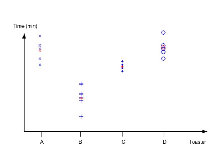
Class Exercise School of Mechatronics Engineering You are an industrial engineer of toaster manufacturing, and would like to test other’s company toaster for their bread cooking time, in order to design the best toaster for your company. The test result is tabulated. Toaster A B C D Test 1 4. 5 2. 5 3. 7 4. 6 Bread cooking time (min) Test 2 Test 3 Test 4 4. 1 3. 6 4. 2 2. 6 3. 0 2. 7 3. 6 3. 4 3. 5 3. 8 4. 2 4. 1 Test 5 3. 8 2. 0 3. 5 4. 0 Compute the mean and standard deviation for each Toaster. Write final value and uncertainties for each Toaster. Sketch the test/measurement in a graph and observe the precision and accuracy. Which one is better?