ENGINEERING OPTIMIZATION Methods and Applications A Ravindran K

ENGINEERING OPTIMIZATION Methods and Applications A. Ravindran, K. M. Ragsdell, G. V. Reklaitis Book Review Page 1

Chapter 4: Linear Programming Part 1: Abu (Sayeem) Reaz Part 2: Rui (Richard) Wang Review Session June 25, 2010 Page 2

Finding the optimum of any given world – how cool is that? ! Page 3

Outline of Part 1 • Formulations • Graphical Solutions • Standard Form • Computer Solutions • Sensitivity Analysis • Applications • Duality Theory Page 4

Outline of Part 1 • Formulations • Graphical Solutions • Standard Form • Computer Solutions • Sensitivity Analysis • Applications • Duality Theory Page 5

What is an LP? An LP has • An objective to find the best value for a system • A set of design variables that represents the system • A list of requirements that draws constraints the design variables The constraints of the system can be expressed as linear equations or inequalities and the objective function is a linear function of the design variables Page 6

Types Linear Program (LP): all variables are real Integer Linear Program (ILP): all variables are integer Mixed Integer Linear Program (MILP): variables are a mix of integer and real number Binary Linear Program (BLP): all variables are binary Page 7

Formulation is the construction of LP models of real problems: • To identify the design/decision variables • Express the constraints of the problem as linear equations or inequalities • Write the objective function to be maximized or minimized as a linear function Page 8

The Wisdom of Linear Programming “Model building is not a science; it is primarily an art that is developed mainly by experience” Page 9

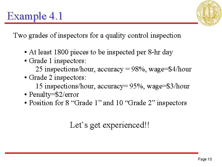
Example 4. 1 Two grades of inspectors for a quality control inspection • At least 1800 pieces to be inspected per 8 -hr day • Grade 1 inspectors: 25 inspections/hour, accuracy = 98%, wage=$4/hour • Grade 2 inspectors: 15 inspections/hour, accuracy= 95%, wage=$3/hour • Penalty=$2/error • Position for 8 “Grade 1” and 10 “Grade 2” inspectors Let’s get experienced!! Page 10

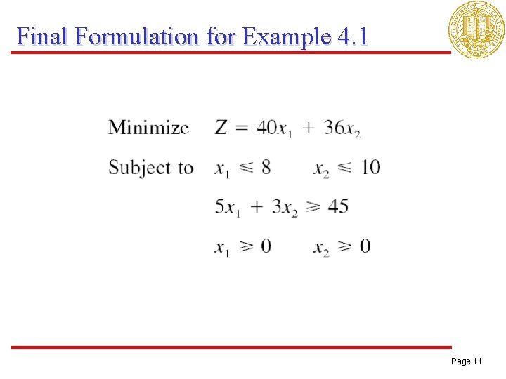
Final Formulation for Example 4. 1 Page 11

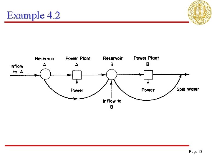
Example 4. 2 Page 12

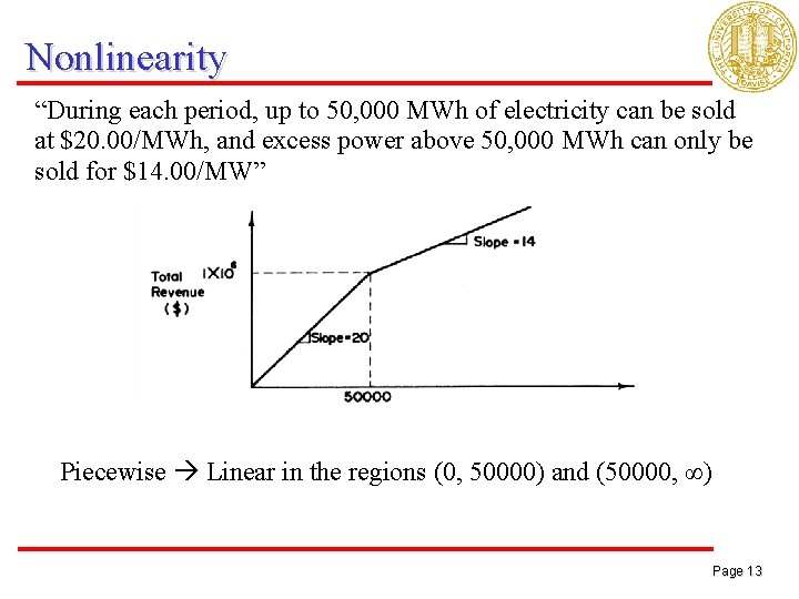
Nonlinearity “During each period, up to 50, 000 MWh of electricity can be sold at $20. 00/MWh, and excess power above 50, 000 MWh can only be sold for $14. 00/MW” Piecewise Linear in the regions (0, 50000) and (50000, ∞) Page 13

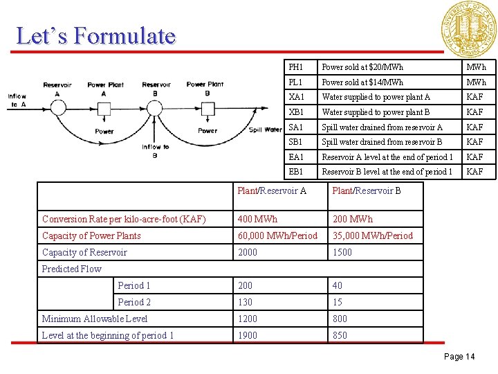
Let’s Formulate PH 1 Power sold at $20/MWh PL 1 Power sold at $14/MWh XA 1 Water supplied to power plant A KAF XB 1 Water supplied to power plant B KAF SA 1 Spill water drained from reservoir A KAF SB 1 Spill water drained from reservoir B KAF EA 1 Reservoir A level at the end of period 1 KAF EB 1 Reservoir B level at the end of period 1 KAF Plant/Reservoir A Plant/Reservoir B Conversion Rate per kilo-acre-foot (KAF) 400 MWh 200 MWh Capacity of Power Plants 60, 000 MWh/Period 35, 000 MWh/Period Capacity of Reservoir 2000 1500 Period 1 200 40 Period 2 130 15 Minimum Allowable Level 1200 800 Level at the beginning of period 1 1900 850 Predicted Flow Page 14

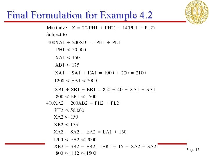
Final Formulation for Example 4. 2 Page 15

Outline of Part 1 • Formulations • Graphical Solutions • Standard Form • Computer Solutions • Sensitivity Analysis • Applications • Duality Theory Page 16

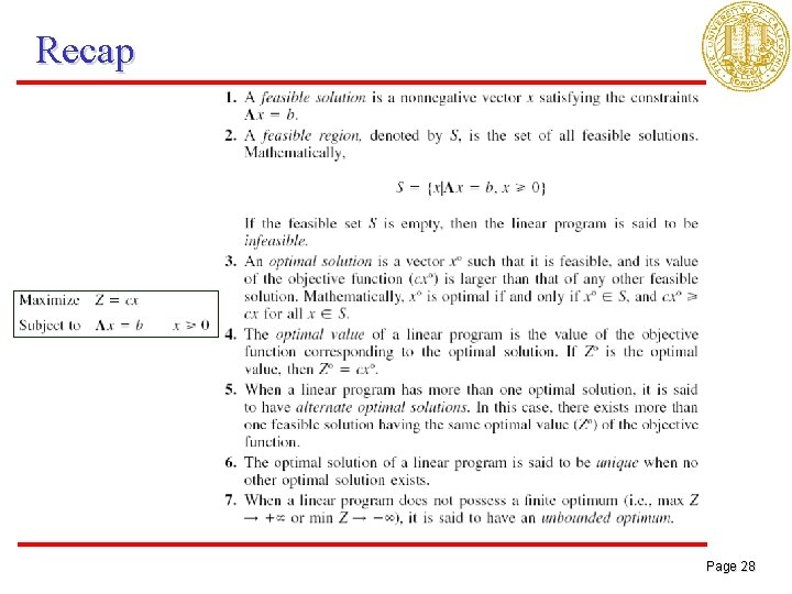
Definitions • Feasible Solution: all possible values of decision variables that satisfy the constraints • Feasible Region: the set of all feasible solutions • Optimal Solution: The best feasible solution • Optimal Value: The value of the objective function corresponding to an optimal solution Page 17

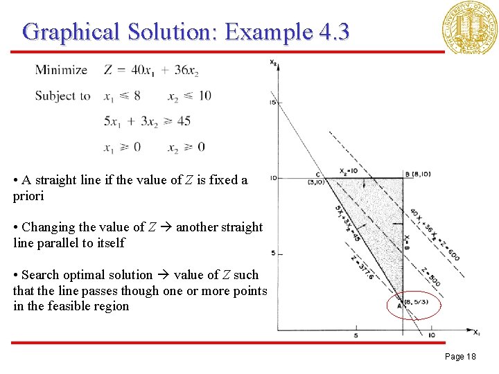
Graphical Solution: Example 4. 3 • A straight line if the value of Z is fixed a priori • Changing the value of Z another straight line parallel to itself • Search optimal solution value of Z such that the line passes though one or more points in the feasible region Page 18

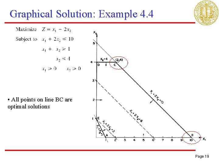
Graphical Solution: Example 4. 4 • All points on line BC are optimal solutions Page 19

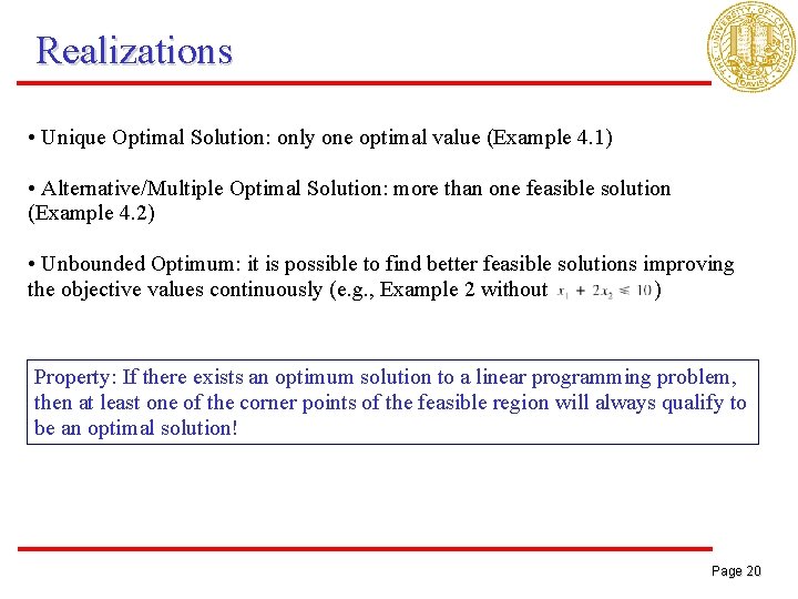
Realizations • Unique Optimal Solution: only one optimal value (Example 4. 1) • Alternative/Multiple Optimal Solution: more than one feasible solution (Example 4. 2) • Unbounded Optimum: it is possible to find better feasible solutions improving the objective values continuously (e. g. , Example 2 without ) Property: If there exists an optimum solution to a linear programming problem, then at least one of the corner points of the feasible region will always qualify to be an optimal solution! Page 20

Outline of Part 1 • Formulations • Graphical Solutions • Standard Form • Computer Solutions • Sensitivity Analysis • Applications • Duality Theory Page 21

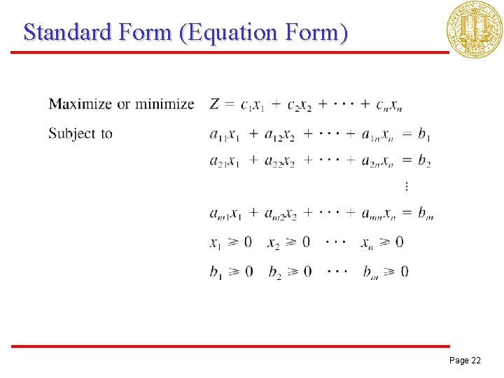
Standard Form (Equation Form) Page 22

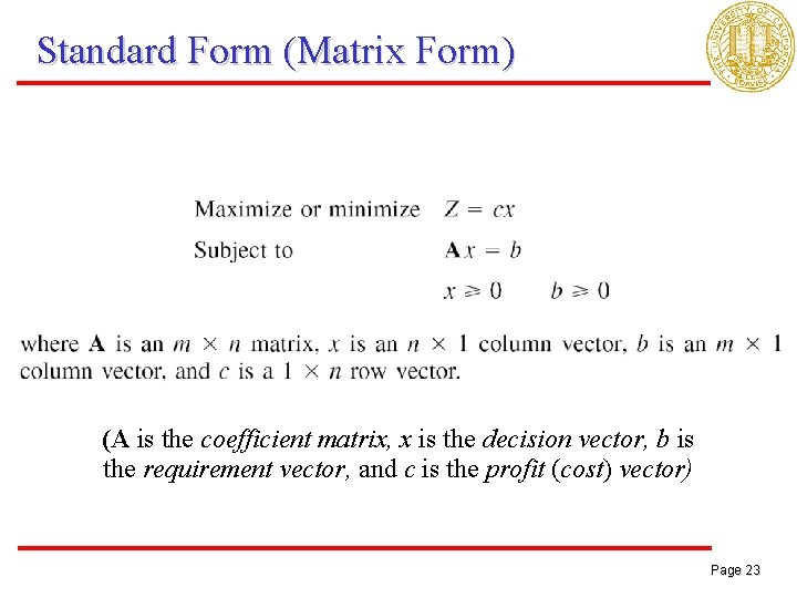
Standard Form (Matrix Form) (A is the coefficient matrix, x is the decision vector, b is the requirement vector, and c is the profit (cost) vector) Page 23

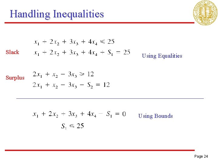
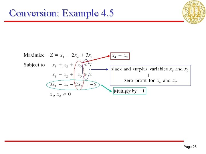
Handling Inequalities Slack Using Equalities Surplus Using Bounds Page 24

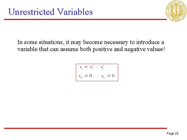
Unrestricted Variables In some situations, it may become necessary to introduce a variable that can assume both positive and negative values! Page 25

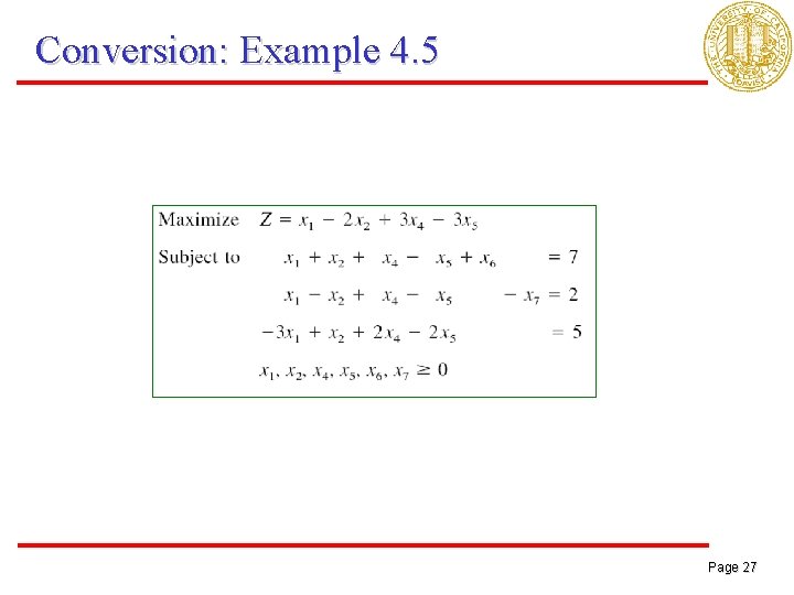
Conversion: Example 4. 5 Page 26

Conversion: Example 4. 5 Page 27

Recap Page 28

Outline of Part 1 • Formulations • Graphical Solutions • Standard Form • Computer Solutions • Sensitivity Analysis • Applications • Duality Theory Page 29

Computer Codes • For small/simple LPs: • Microsoft Excel • For High-End LP: • OSL from IBM • ILOG CPLEX • OB 1 in XMP Software • Modeling Language: • GAMS (General Algebraic Modeling System) • AMPL (A Mathematical Programming Language) • Internet • http: / /www. ece. northwestern. edu/otc Page 30

Outline of Part 1 • Formulations • Graphical Solutions • Standard Form • Computer Solutions • Sensitivity Analysis • Applications • Duality Theory Page 31

Sensitivity Analysis • Variation in the values of the data coefficients changes the LP problem, which may in turn affect the optimal solution. • The study of how the optimal solution will change with changes in the input (data) coefficients is known as sensitivity analysis or post-optimality analysis. • Why? • Some parameters may be controllable better optimal value • Data coefficients from statistical estimation identify the one that effects the objective value most obtain better estimates Page 32

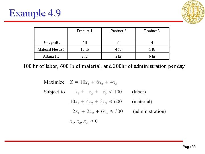
Example 4. 9 Product 1 Product 2 Product 3 Unit profit 10 6 4 Material Needed 10 lb 4 lb 5 lb Admin Hr 2 hr 6 hr 100 hr of labor, 600 lb of material, and 300 hr of administration per day Page 33

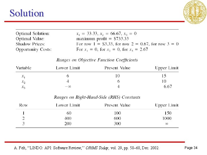
Solution A. Felt, ‘‘LINDO: API: Software Review, ’’ OR/MS Today, vol. 29, pp. 58– 60, Dec. 2002. Page 34

Outline of Part 1 • Formulations • Graphical Solutions • Standard Form • Computer Solutions • Sensitivity Analysis • Applications • Duality Theory Page 35

Applications of LP For any optimization problem in linear form with feasible solution time! Page 36

Outline of Part 1 • Formulations • Graphical Solutions • Standard Form • Computer Solutions • Sensitivity Analysis • Applications • Duality Theory (Additional Topic) Page 37

Duality of LP Every linear programming problem has an associated linear program called its dual such that a solution to the original linear program also gives a solution to its dual Solve one, get one free!! Page 38

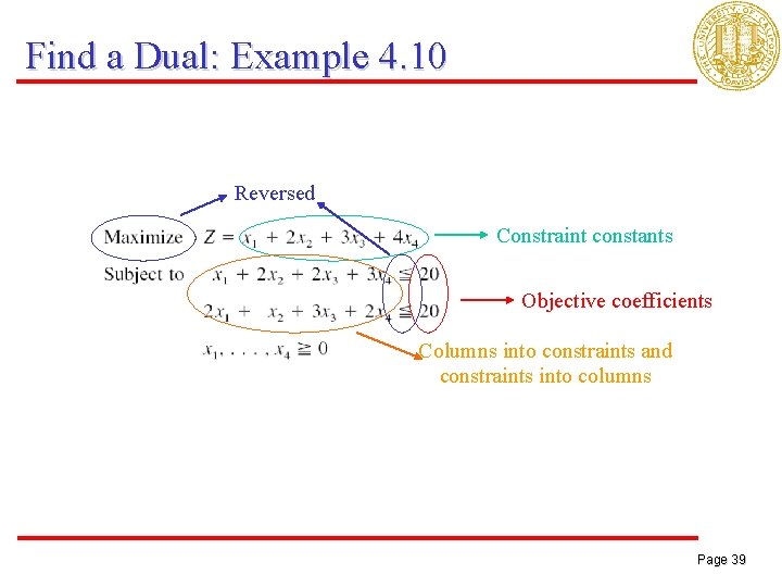
Find a Dual: Example 4. 10 Reversed Constraint constants Objective coefficients Columns into constraints and constraints into columns Page 39

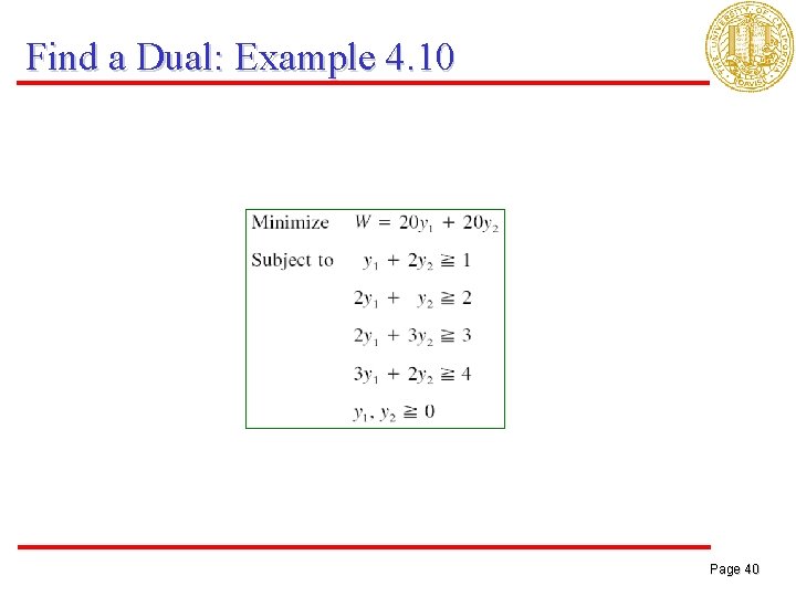
Find a Dual: Example 4. 10 Page 40

Some Tricks • “Binarization” • If • OR • AND • Finding Range • Finding the value of a variable http: //networks. cs. ucdavis. edu/ppt/group_meeting_22 may 2009. pdf Page 41

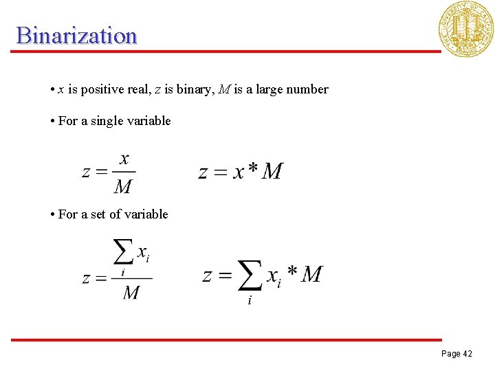
Binarization • x is positive real, z is binary, M is a large number • For a single variable • For a set of variable Page 42

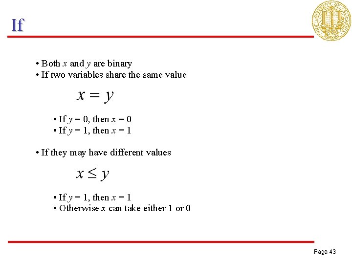
If • Both x and y are binary • If two variables share the same value • If y = 0, then x = 0 • If y = 1, then x = 1 • If they may have different values • If y = 1, then x = 1 • Otherwise x can take either 1 or 0 Page 43

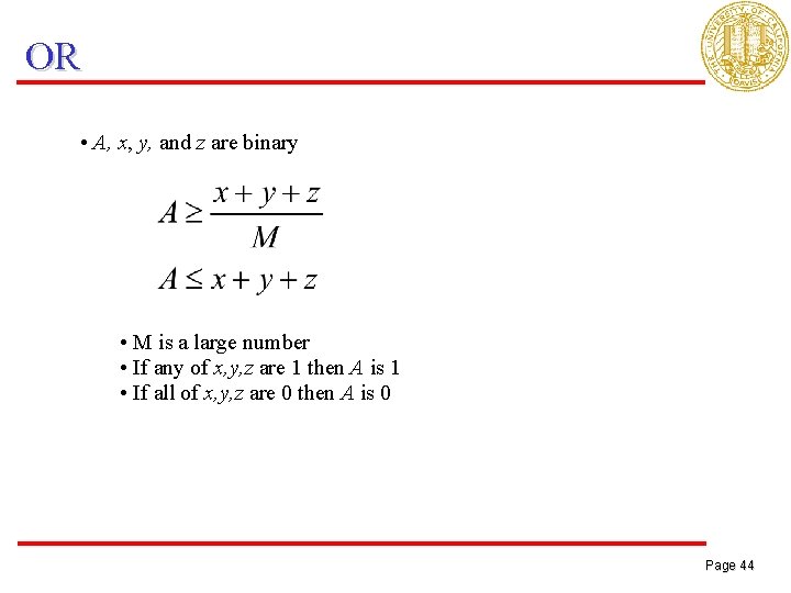
OR • A, x, y, and z are binary • M is a large number • If any of x, y, z are 1 then A is 1 • If all of x, y, z are 0 then A is 0 Page 44

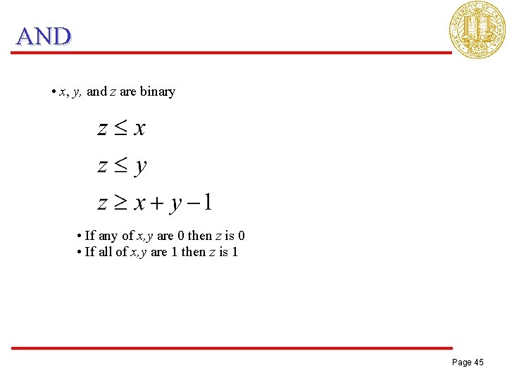
AND • x, y, and z are binary • If any of x, y are 0 then z is 0 • If all of x, y are 1 then z is 1 Page 45

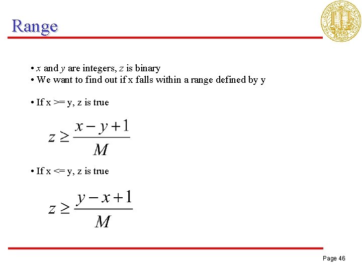
Range • x and y are integers, z is binary • We want to find out if x falls within a range defined by y • If x >= y, z is true • If x <= y, z is true Page 46

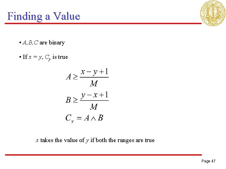
Finding a Value • A, B, C are binary • If x = y, Cy is true x takes the value of y if both the ranges are true Page 47

Thank You! Now Part 2 begins…. Page 48