ENGINEERING OPTIMIZATION Methods and Applications A Ravindran K

ENGINEERING OPTIMIZATION Methods and Applications A. Ravindran, K. M. Ragsdell, G. V. Reklaitis Chapter 8: Linearization Methods for Constrained Problems Book Review Presented by Kartik Pandit July 23, 2010 1

Outline • Introduction • Direct Use of Successive Linear Programs – Linearly Constrained Case – General Nonlinear Programming Case • Separable Programming – Single-Variable Functions – Multivariable Separable Functions – Linear Programming Solutions of Separable – Problems 2

Introduction 3

Introduction • Efficient algorithms exist for two problem classes: – Unconstrained problems – Completely linear constrained problems • Most approaches to solve the general problem of non-linear objective functions with non-linear constraints exploit techniques that solve the “easy” problems. 4

Introduction • The basic Idea: 1. Use linear functions to approximate both the objective function as well as the constraints (Linearization). 2. Employ LP algorithms to solve this new linear program. 5

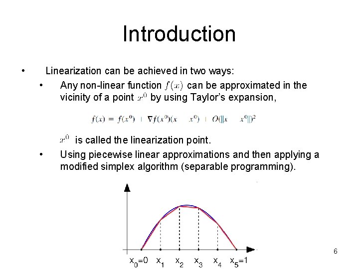
Introduction • Linearization can be achieved in two ways: • Any non-linear function can be approximated in the vicinity of a point by using Taylor’s expansion, • is called the linearization point. Using piecewise linear approximations and then applying a modified simplex algorithm (separable programming). 6

8. 1 Direct Use of Successive Linear Programs 7

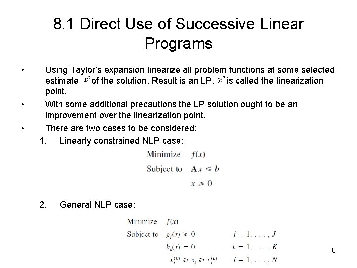
8. 1 Direct Use of Successive Linear Programs • • • Using Taylor’s expansion linearize all problem functions at some selected estimate of the solution. Result is an LP. is called the linearization point. With some additional precautions the LP solution ought to be an improvement over the linearization point. There are two cases to be considered: 1. Linearly constrained NLP case: 2. General NLP case: 8

8. 1. 1 Direct Use of Successive Linear Programs: Linearly constrained NLP case 9

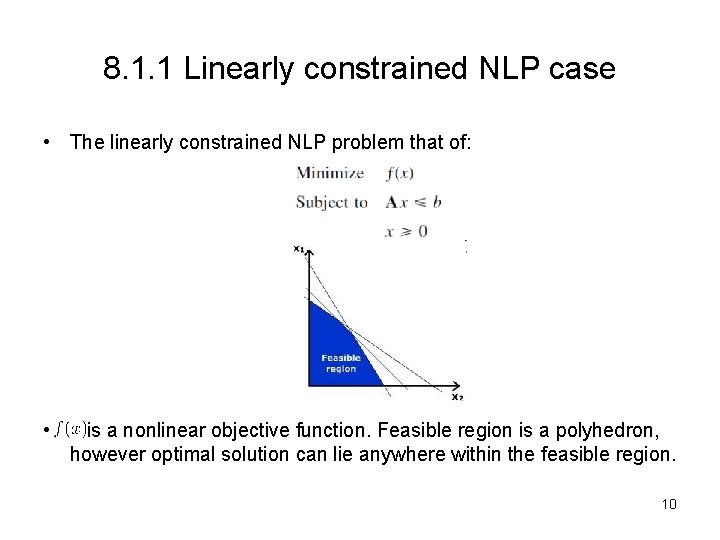
8. 1. 1 Linearly constrained NLP case • The linearly constrained NLP problem that of: • is a nonlinear objective function. Feasible region is a polyhedron, however optimal solution can lie anywhere within the feasible region. 10

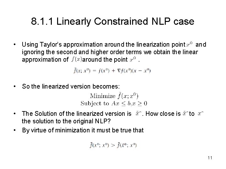
8. 1. 1 Linearly Constrained NLP case • Using Taylor’s approximation around the linearization point and ignoring the second and higher order terms we obtain the linear approximation of around the point. • So the linearized version becomes: • The Solution of the linearized version is. How close is the solution to the original NLP? • By virtue of minimization it must be true that to 11

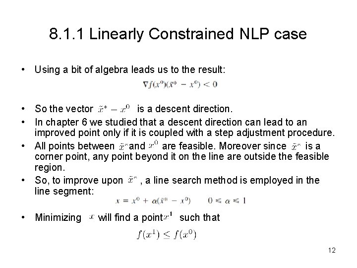
8. 1. 1 Linearly Constrained NLP case • Using a bit of algebra leads us to the result: • So the vector is a descent direction. • In chapter 6 we studied that a descent direction can lead to an improved point only if it is coupled with a step adjustment procedure. • All points between and are feasible. Moreover since is a corner point, any point beyond it on the line are outside the feasible region. • So, to improve upon , a line search method is employed in the line segment: • Minimizing will find a point such that 12

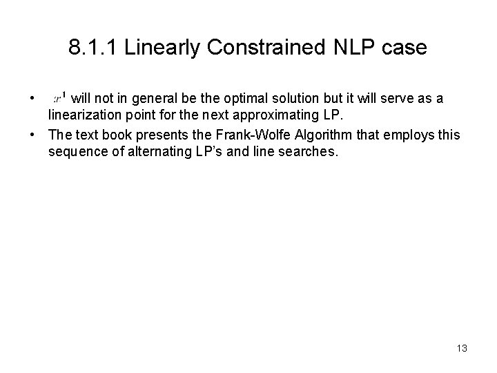
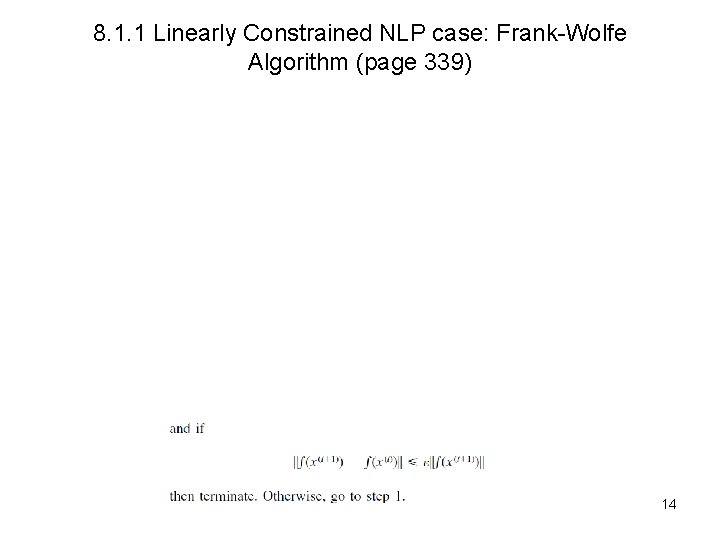
8. 1. 1 Linearly Constrained NLP case • will not in general be the optimal solution but it will serve as a linearization point for the next approximating LP. • The text book presents the Frank-Wolfe Algorithm that employs this sequence of alternating LP’s and line searches. 13

8. 1. 1 Linearly Constrained NLP case: Frank-Wolfe Algorithm (page 339) 14

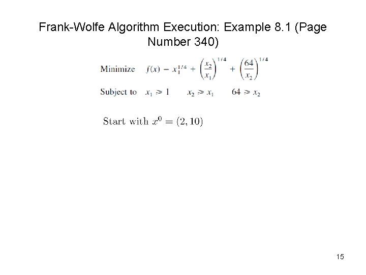
Frank-Wolfe Algorithm Execution: Example 8. 1 (Page Number 340) 15

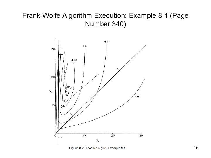
Frank-Wolfe Algorithm Execution: Example 8. 1 (Page Number 340) 16

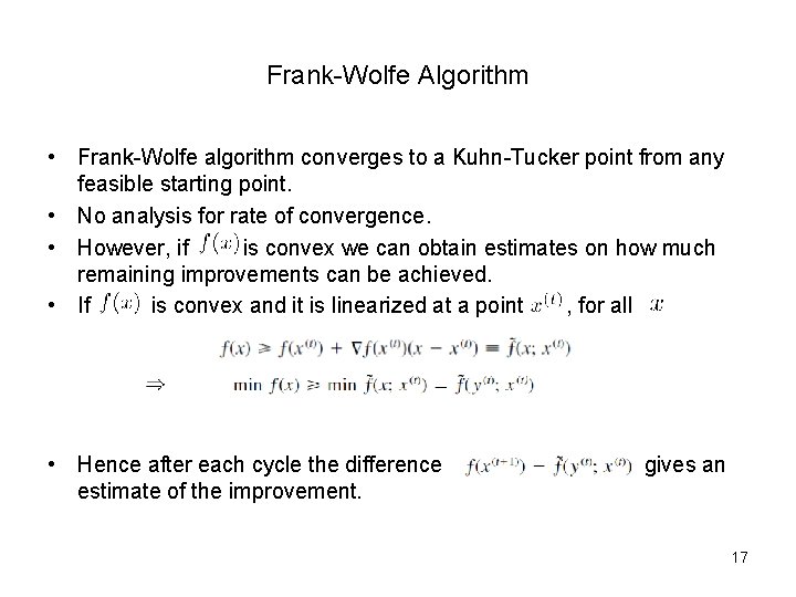
Frank-Wolfe Algorithm • Frank-Wolfe algorithm converges to a Kuhn-Tucker point from any feasible starting point. • No analysis for rate of convergence. • However, if is convex we can obtain estimates on how much remaining improvements can be achieved. • If is convex and it is linearized at a point , for all • Hence after each cycle the difference estimate of the improvement. gives an 17

8. 1. 2 Direct Use of Successive Linear Programs: General NLP case 18

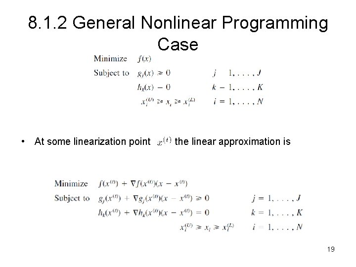
8. 1. 2 General Nonlinear Programming Case • At some linearization point the linear approximation is 19

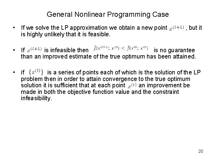
General Nonlinear Programming Case • If we solve the LP approximation we obtain a new point is highly unlikely that it is feasible. , but it • If is infeasible then is no guarantee than an improved estimate of the true optimum has been attained. • if is a series of points each of which is the solution of the LP problem then in order to attain convergence to the true optimum solution it is sufficient that at each point an improvement be made in both the objective function value and the constraint infeasibility. 20

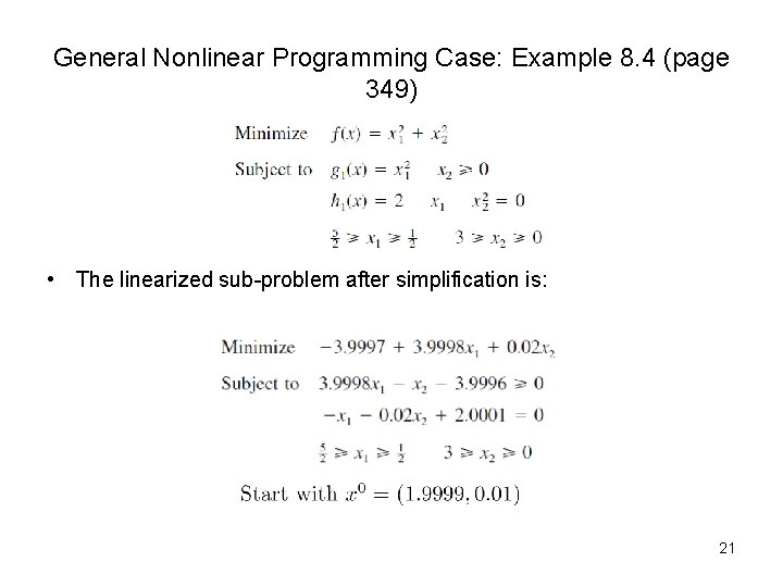
General Nonlinear Programming Case: Example 8. 4 (page 349) • The linearized sub-problem after simplification is: 21

Example 8. 4 22

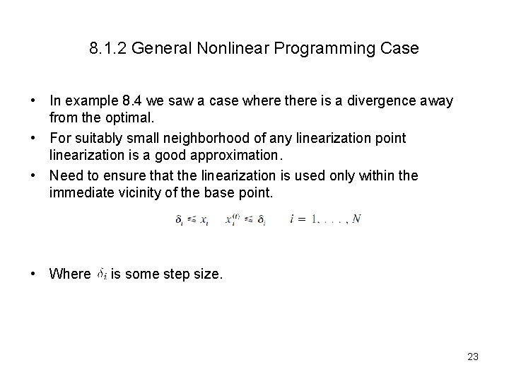
8. 1. 2 General Nonlinear Programming Case • In example 8. 4 we saw a case where there is a divergence away from the optimal. • For suitably small neighborhood of any linearization point linearization is a good approximation. • Need to ensure that the linearization is used only within the immediate vicinity of the base point. • Where is some step size. 23

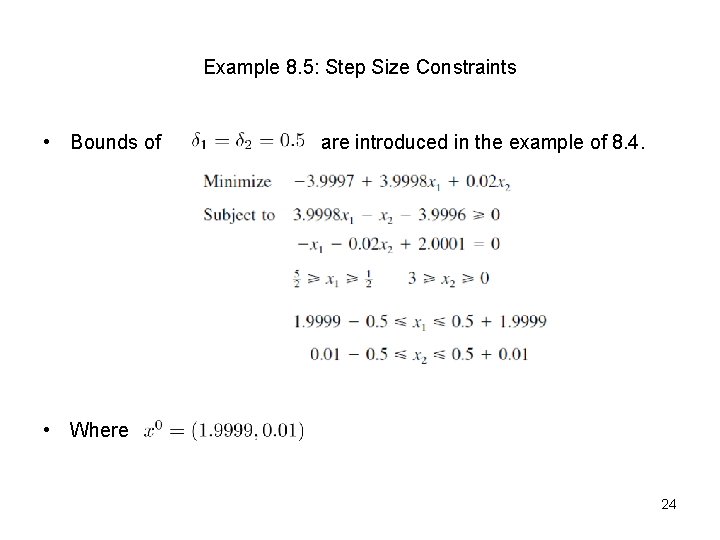
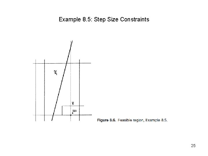
Example 8. 5: Step Size Constraints • Bounds of are introduced in the example of 8. 4. • Where 24

Example 8. 5: Step Size Constraints 25

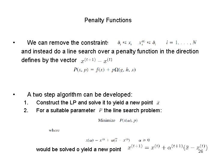
Penalty Functions • • We can remove the constraints and instead do a line search over a penalty function in the direction defines by the vector A two step algorithm can be developed: 1. 2. Construct the LP and solve it to yield a new point For a suitable parameter the line search problem: would be solved o yield a new point 26

8. 2 Separable Programming 27

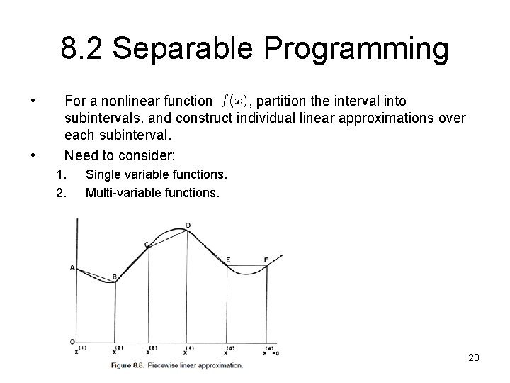
8. 2 Separable Programming • • For a nonlinear function , partition the interval into subintervals. and construct individual linear approximations over each subinterval. Need to consider: 1. 2. Single variable functions. Multi-variable functions. 28

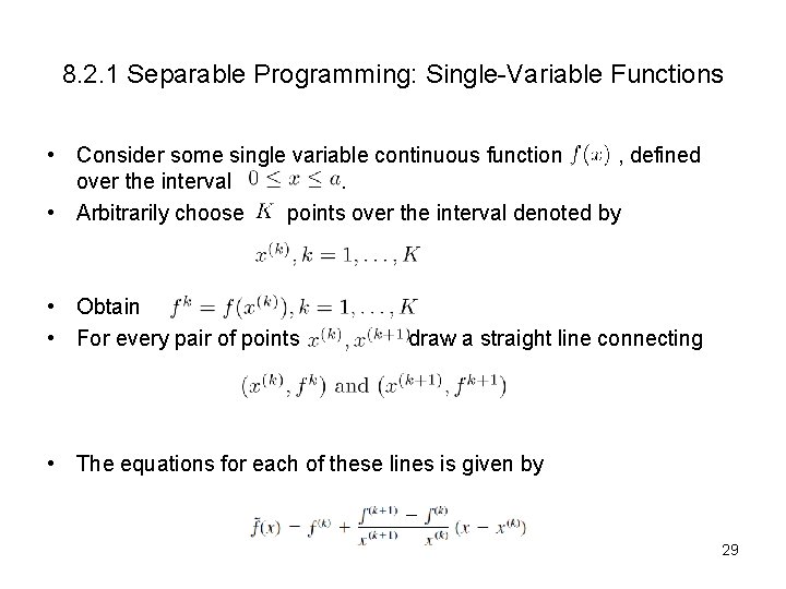
8. 2. 1 Separable Programming: Single-Variable Functions • Consider some single variable continuous function , defined over the interval. • Arbitrarily choose points over the interval denoted by • Obtain • For every pair of points draw a straight line connecting • The equations for each of these lines is given by 29

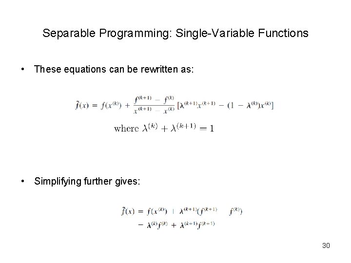
Separable Programming: Single-Variable Functions • These equations can be rewritten as: • Simplifying further gives: 30

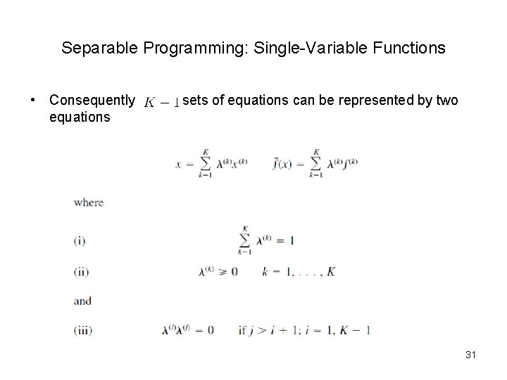
Separable Programming: Single-Variable Functions • Consequently equations sets of equations can be represented by two 31

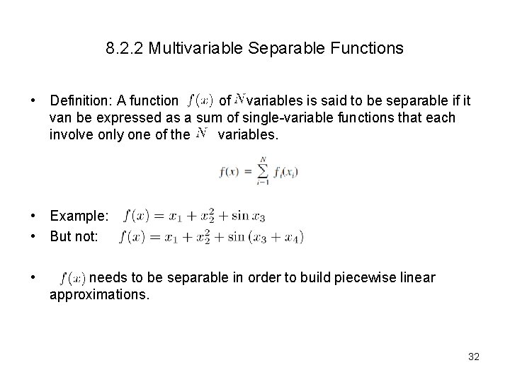
8. 2. 2 Multivariable Separable Functions • Definition: A function of variables is said to be separable if it van be expressed as a sum of single-variable functions that each involve only one of the variables. • Example: • But not: • needs to be separable in order to build piecewise linear approximations. 32

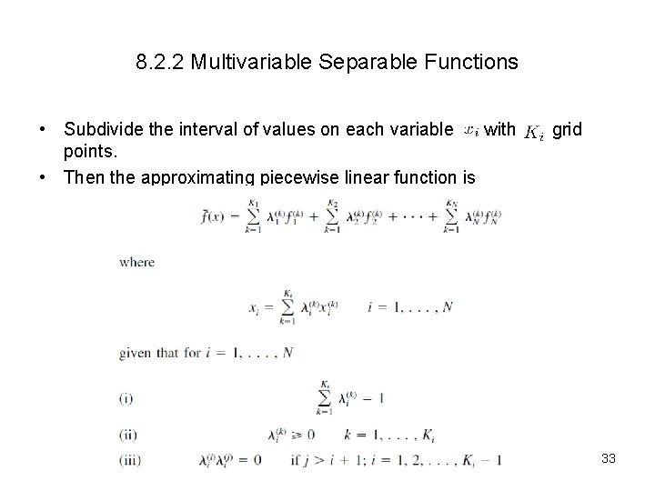
8. 2. 2 Multivariable Separable Functions • Subdivide the interval of values on each variable with points. • Then the approximating piecewise linear function is grid 33

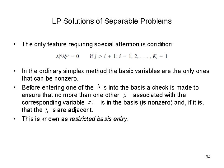
LP Solutions of Separable Problems • The only feature requiring special attention is condition: • In the ordinary simplex method the basic variables are the only ones that can be nonzero. • Before entering one of the ‘s into the basis a check is made to ensure that no more than one other associated with the corresponding variable is in the basis (is nonzero) and, if it is, that the ‘s are adjacent. • This is known as restricted basis entry. 34

End 35