ECE 250 Algorithms and Data Structures Sorting algorithms

ECE 250 Algorithms and Data Structures Sorting algorithms Douglas Wilhelm Harder, M. Math. LEL Department of Electrical and Computer Engineering University of Waterloo, Ontario, Canada ece. uwaterloo. ca dwharder@alumni. uwaterloo. ca © 2006 -2013 by Douglas Wilhelm Harder. Some rights reserved.

Sorting algorithms 2 Outline In this topic, we will introduce sorting, including: – – – Definitions Assumptions In-place sorting Sorting techniques and strategies Overview of run times Lower bound on run times Define inversions and use this as a measure of unsortedness

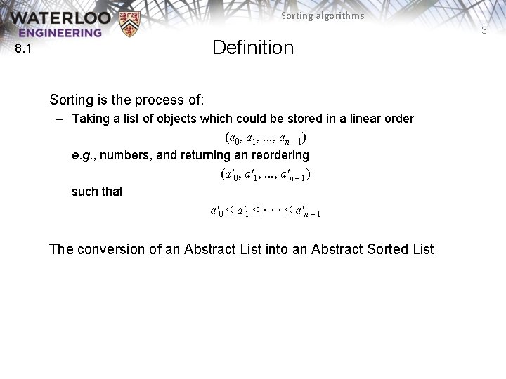
Sorting algorithms 3 Definition 8. 1 Sorting is the process of: – Taking a list of objects which could be stored in a linear order (a 0, a 1, . . . , an – 1) e. g. , numbers, and returning an reordering (a'0, a'1, . . . , a'n – 1) such that a'0 ≤ a'1 ≤ · · · ≤ a'n – 1 The conversion of an Abstract List into an Abstract Sorted List

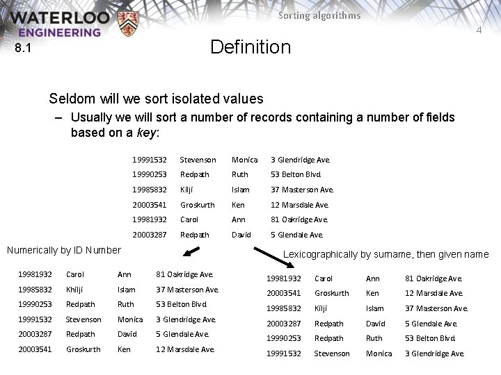
Sorting algorithms 4 Definition 8. 1 Seldom will we sort isolated values – Usually we will sort a number of records containing a number of fields based on a key: 19991532 Stevenson Monica 3 Glendridge Ave. 19990253 Redpath Ruth 53 Belton Blvd. 19985832 Kilji Islam 37 Masterson Ave. 20003541 Groskurth Ken 12 Marsdale Ave. 19981932 Carol Ann 81 Oakridge Ave. 20003287 Redpath David 5 Glendale Ave. Numerically by ID Number Lexicographically by surname, then given name 19981932 Carol Ann 81 Oakridge Ave. 19985832 Khilji Islam 37 Masterson Ave. 20003541 Groskurth Ken 12 Marsdale Ave. 19990253 Redpath Ruth 53 Belton Blvd. 19985832 Kilji Islam 37 Masterson Ave. 19991532 Stevenson Monica 3 Glendridge Ave. 20003287 Redpath David 5 Glendale Ave. 19990253 Redpath Ruth 53 Belton Blvd. 20003541 Groskurth Ken 12 Marsdale Ave. 19991532 Stevenson Monica 3 Glendridge Ave.

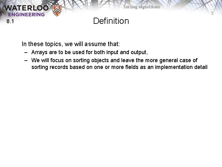
Sorting algorithms 5 8. 1 Definition In these topics, we will assume that: – Arrays are to be used for both input and output, – We will focus on sorting objects and leave the more general case of sorting records based on one or more fields as an implementation detail

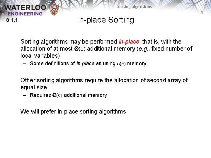
Sorting algorithms 6 8. 1. 1 In-place Sorting algorithms may be performed in-place, that is, with the allocation of at most Q(1) additional memory (e. g. , fixed number of local variables) – Some definitions of in place as using o(n) memory Other sorting algorithms require the allocation of second array of equal size – Requires Q(n) additional memory We will prefer in-place sorting algorithms

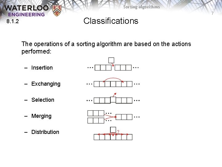
Sorting algorithms 7 Classifications 8. 1. 2 The operations of a sorting algorithm are based on the actions performed: – Insertion – Exchanging – Selection – Merging – Distribution

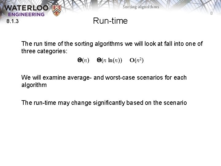
Sorting algorithms 8 8. 1. 3 Run-time The run time of the sorting algorithms we will look at fall into one of three categories: Q(n) Q(n ln(n)) O(n 2) We will examine average- and worst-case scenarios for each algorithm The run-time may change significantly based on the scenario

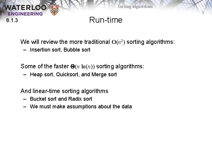
Sorting algorithms 9 8. 1. 3 Run-time We will review the more traditional O(n 2) sorting algorithms: – Insertion sort, Bubble sort Some of the faster Q(n ln(n)) sorting algorithms: – Heap sort, Quicksort, and Merge sort And linear-time sorting algorithms – Bucket sort and Radix sort – We must make assumptions about the data

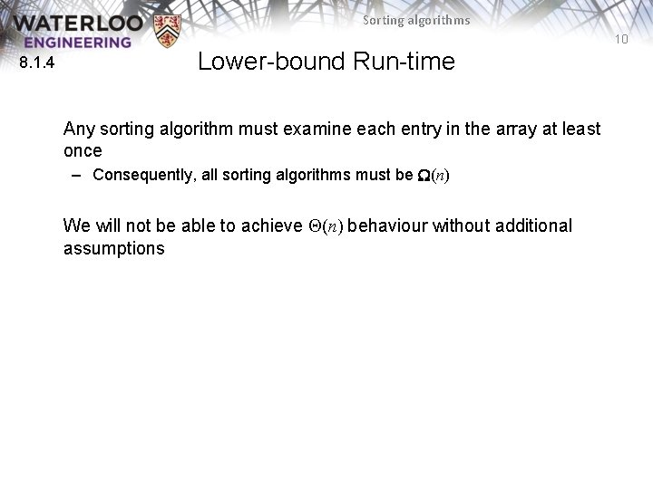
Sorting algorithms 10 8. 1. 4 Lower-bound Run-time Any sorting algorithm must examine each entry in the array at least once – Consequently, all sorting algorithms must be W(n) We will not be able to achieve Q(n) behaviour without additional assumptions

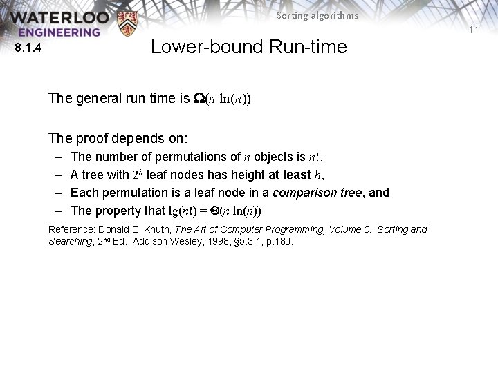
Sorting algorithms 11 Lower-bound Run-time 8. 1. 4 The general run time is W(n ln(n)) The proof depends on: – – The number of permutations of n objects is n!, A tree with 2 h leaf nodes has height at least h, Each permutation is a leaf node in a comparison tree, and The property that lg(n!) = Q(n ln(n)) Reference: Donald E. Knuth, The Art of Computer Programming, Volume 3: Sorting and Searching, 2 nd Ed. , Addison Wesley, 1998, § 5. 3. 1, p. 180.

Sorting algorithms 12 8. 1. 5 Optimal Sorting Algorithms The next seven topics will cover seven common sorting algorithms – There is no optimal sorting algorithm which can be used in all places – Under various circumstances, different sorting algorithms will deliver optimal run-time and memory-allocation requirements

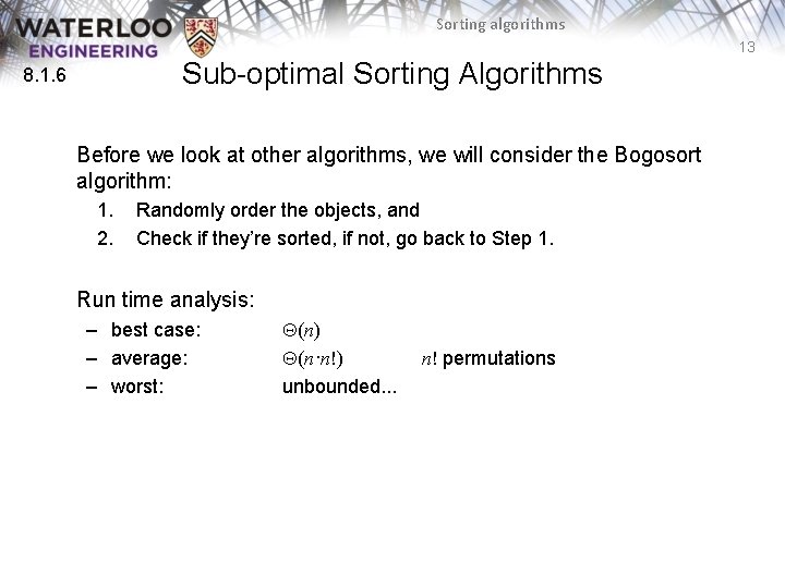
Sorting algorithms 13 Sub-optimal Sorting Algorithms 8. 1. 6 Before we look at other algorithms, we will consider the Bogosort algorithm: 1. 2. Randomly order the objects, and Check if they’re sorted, if not, go back to Step 1. Run time analysis: – best case: – average: – worst: Q(n) Q(n·n!) unbounded. . . n! permutations

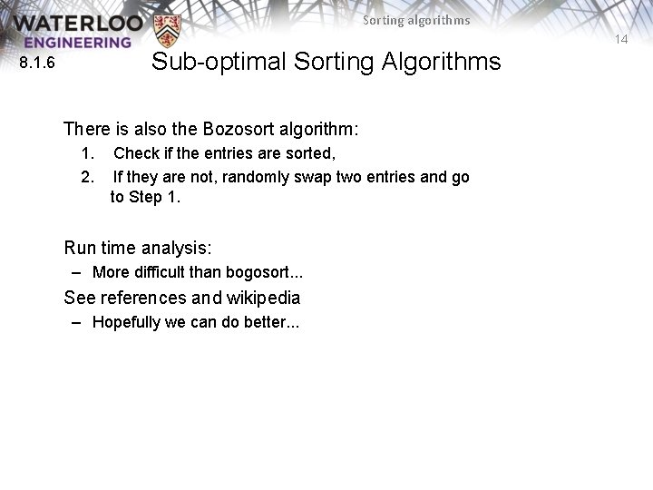
Sorting algorithms 14 Sub-optimal Sorting Algorithms 8. 1. 6 There is also the Bozosort algorithm: 1. 2. Check if the entries are sorted, If they are not, randomly swap two entries and go to Step 1. Run time analysis: – More difficult than bogosort. . . See references and wikipedia – Hopefully we can do better. . .

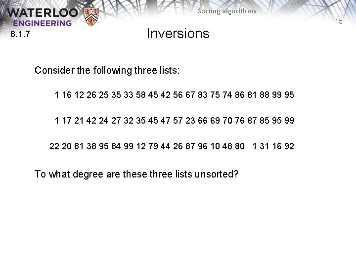
Sorting algorithms 15 8. 1. 7 Inversions Consider the following three lists: 1 16 12 26 25 35 33 58 45 42 56 67 83 75 74 86 81 88 99 95 1 17 21 42 24 27 32 35 45 47 57 23 66 69 70 76 87 85 95 99 22 20 81 38 95 84 99 12 79 44 26 87 96 10 48 80 1 31 16 92 To what degree are these three lists unsorted?

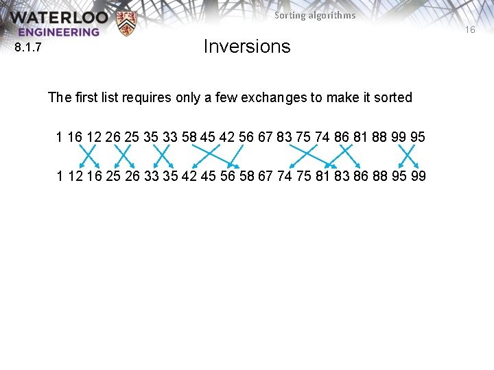
Sorting algorithms 16 8. 1. 7 Inversions The first list requires only a few exchanges to make it sorted 1 16 12 26 25 35 33 58 45 42 56 67 83 75 74 86 81 88 99 95 1 12 16 25 26 33 35 42 45 56 58 67 74 75 81 83 86 88 95 99

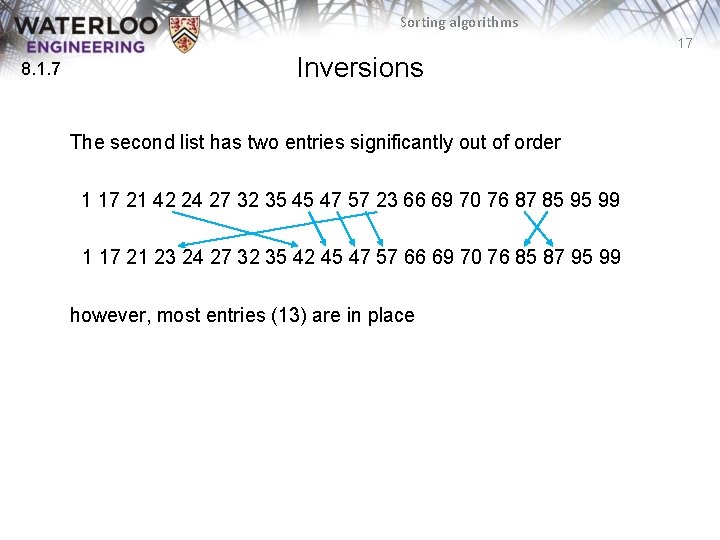
Sorting algorithms 17 8. 1. 7 Inversions The second list has two entries significantly out of order 1 17 21 42 24 27 32 35 45 47 57 23 66 69 70 76 87 85 95 99 1 17 21 23 24 27 32 35 42 45 47 57 66 69 70 76 85 87 95 99 however, most entries (13) are in place

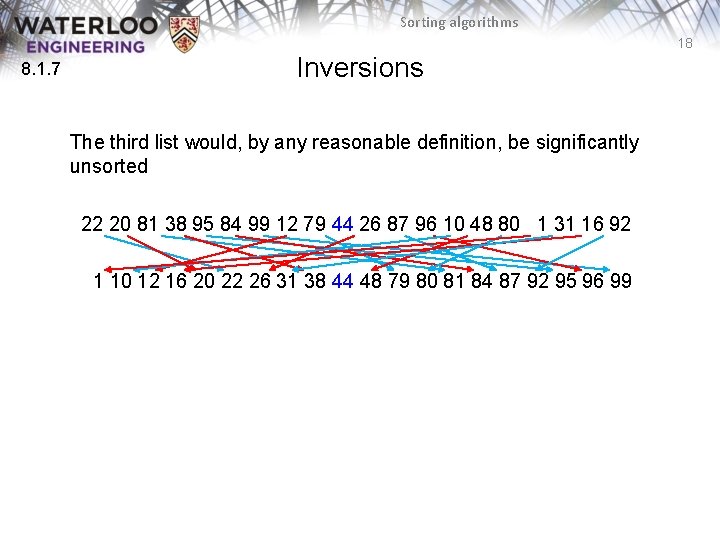
Sorting algorithms 18 8. 1. 7 Inversions The third list would, by any reasonable definition, be significantly unsorted 22 20 81 38 95 84 99 12 79 44 26 87 96 10 48 80 1 31 16 92 1 10 12 16 20 22 26 31 38 44 48 79 80 81 84 87 92 95 96 99

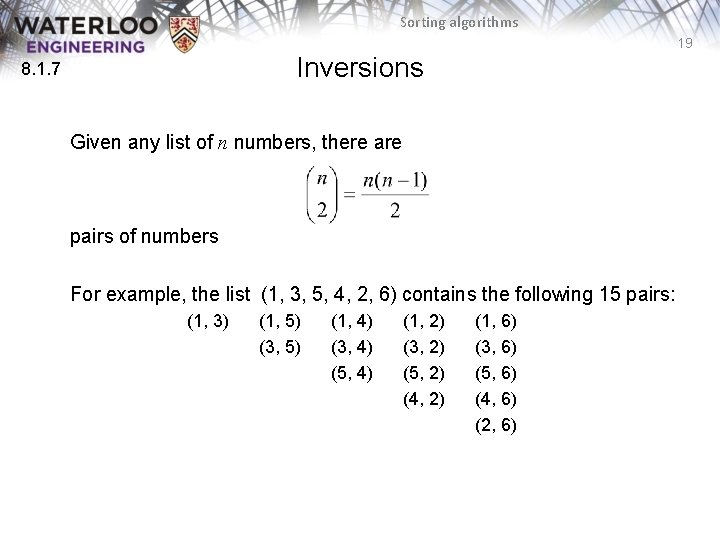
Sorting algorithms 19 Inversions 8. 1. 7 Given any list of n numbers, there are pairs of numbers For example, the list (1, 3, 5, 4, 2, 6) contains the following 15 pairs: (1, 3) (1, 5) (3, 5) (1, 4) (3, 4) (5, 4) (1, 2) (3, 2) (5, 2) (4, 2) (1, 6) (3, 6) (5, 6) (4, 6) (2, 6)

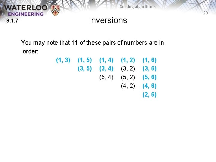
Sorting algorithms 20 8. 1. 7 Inversions You may note that 11 of these pairs of numbers are in order: (1, 3) (1, 5) (1, 4) (1, 2) (1, 6) (3, 5) (3, 4) (3, 2) (3, 6) (5, 4) (5, 2) (5, 6) (4, 2) (4, 6) (2, 6)

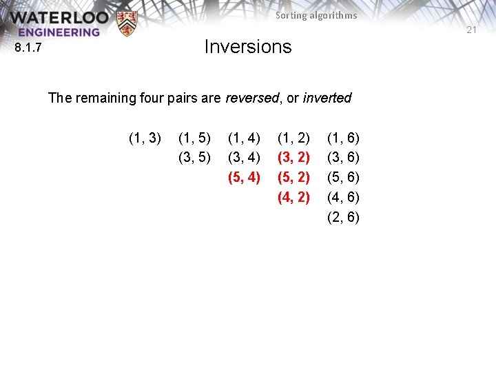
Sorting algorithms 21 Inversions 8. 1. 7 The remaining four pairs are reversed, or inverted (1, 3) (1, 5) (3, 5) (1, 4) (3, 4) (5, 4) (1, 2) (3, 2) (5, 2) (4, 2) (1, 6) (3, 6) (5, 6) (4, 6) (2, 6)

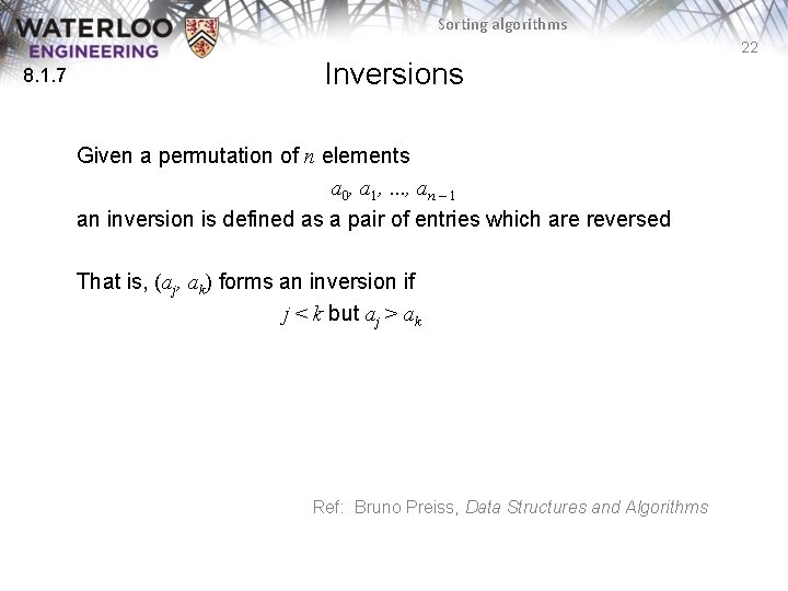
Sorting algorithms 22 8. 1. 7 Inversions Given a permutation of n elements a 0, a 1, . . . , an – 1 an inversion is defined as a pair of entries which are reversed That is, (aj, ak) forms an inversion if j < k but aj > ak Ref: Bruno Preiss, Data Structures and Algorithms

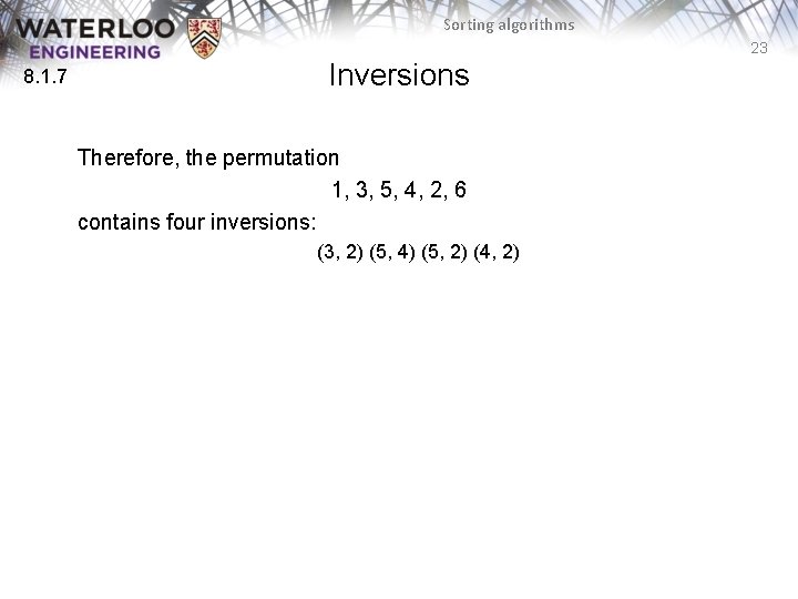
Sorting algorithms 23 8. 1. 7 Inversions Therefore, the permutation 1, 3, 5, 4, 2, 6 contains four inversions: (3, 2) (5, 4) (5, 2) (4, 2)

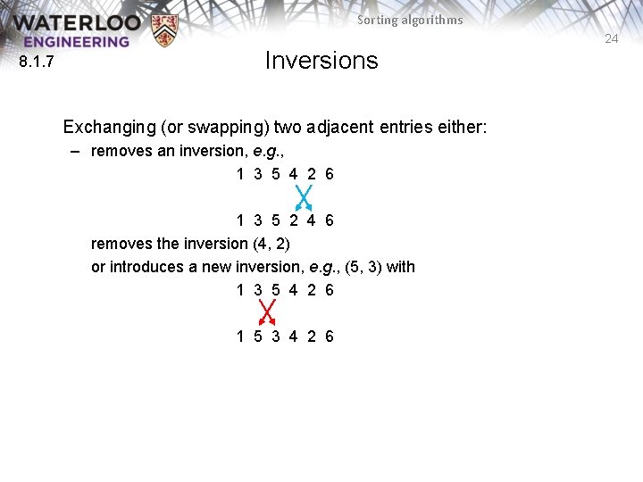
Sorting algorithms 24 8. 1. 7 Inversions Exchanging (or swapping) two adjacent entries either: – removes an inversion, e. g. , 1 3 5 4 2 6 1 3 5 2 4 6 removes the inversion (4, 2) or introduces a new inversion, e. g. , (5, 3) with 1 3 5 4 2 6 1 5 3 4 2 6

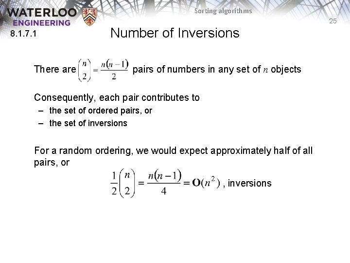
Sorting algorithms 25 Number of Inversions 8. 1. 7. 1 There are pairs of numbers in any set of n objects Consequently, each pair contributes to – the set of ordered pairs, or – the set of inversions For a random ordering, we would expect approximately half of all pairs, or , inversions

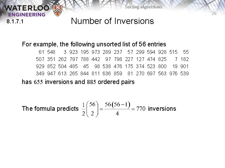
Sorting algorithms 26 Number of Inversions 8. 1. 7. 1 For example, the following unsorted list of 56 entries 61 507 929 349 548 3 923 195 973 289 237 57 299 594 351 262 797 788 442 97 798 227 127 474 852 504 485 45 98 538 476 175 374 523 947 613 265 844 811 636 859 81 270 697 928 515 55 825 7 182 800 19 901 563 976 539 has 655 inversions and 885 ordered pairs The formula predicts inversions

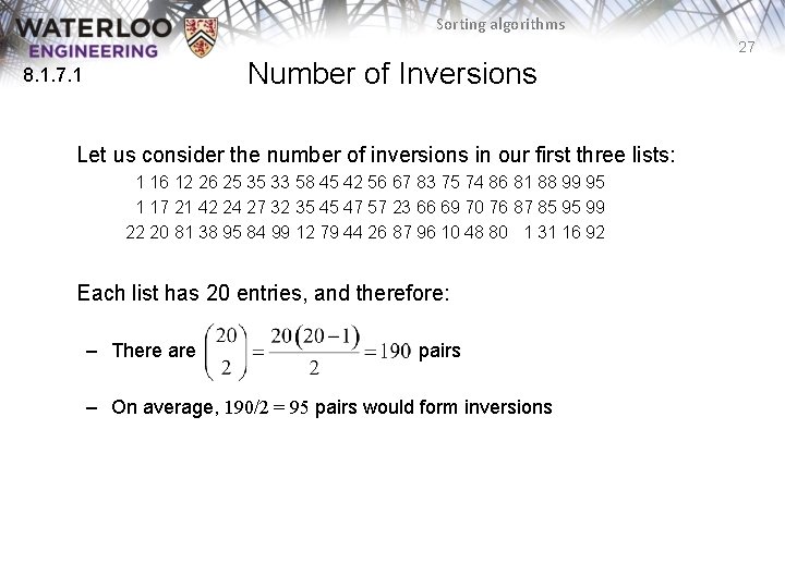
Sorting algorithms 27 Number of Inversions 8. 1. 7. 1 Let us consider the number of inversions in our first three lists: 1 16 12 26 25 35 33 58 45 42 56 67 83 75 74 86 81 88 99 95 1 17 21 42 24 27 32 35 45 47 57 23 66 69 70 76 87 85 95 99 22 20 81 38 95 84 99 12 79 44 26 87 96 10 48 80 1 31 16 92 Each list has 20 entries, and therefore: – There are pairs – On average, 190/2 = 95 pairs would form inversions

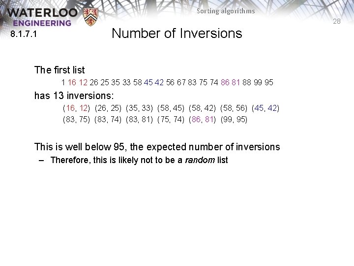
Sorting algorithms 28 Number of Inversions 8. 1. 7. 1 The first list 1 16 12 26 25 35 33 58 45 42 56 67 83 75 74 86 81 88 99 95 has 13 inversions: (16, 12) (26, 25) (35, 33) (58, 45) (58, 42) (58, 56) (45, 42) (83, 75) (83, 74) (83, 81) (75, 74) (86, 81) (99, 95) This is well below 95, the expected number of inversions – Therefore, this is likely not to be a random list

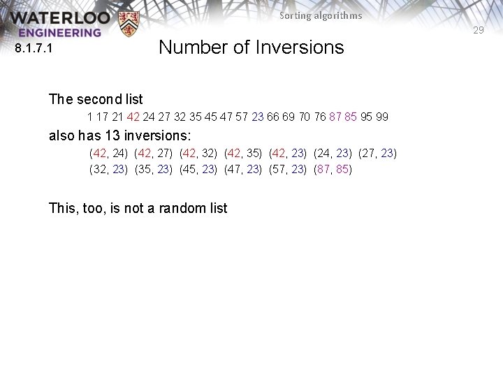
Sorting algorithms 29 Number of Inversions 8. 1. 7. 1 The second list 1 17 21 42 24 27 32 35 45 47 57 23 66 69 70 76 87 85 95 99 also has 13 inversions: (42, 24) (42, 27) (42, 32) (42, 35) (42, 23) (24, 23) (27, 23) (32, 23) (35, 23) (47, 23) (57, 23) (87, 85) This, too, is not a random list

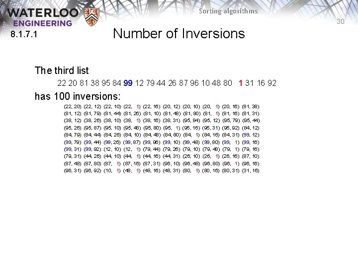
Sorting algorithms 30 Number of Inversions 8. 1. 7. 1 The third list 22 20 81 38 95 84 99 12 79 44 26 87 96 10 48 80 1 31 16 92 has 100 inversions: (22, 20) (81, 12) (38, 12) (95, 26) (84, 79) (99, 31) (79, 31) (87, 48) (96, 31) (22, 12) (81, 79) (38, 26) (95, 87) (84, 44) (99, 92) (44, 26) (87, 80) (96, 92) (22, 10) (81, 44) (38, 10) (95, 10) (84, 26) (99, 26) (12, 10) (44, 10) (87, 1) (10, 1) (22, 1) (81, 26) (38, 1) (95, 48) (84, 10) (99, 87) (12, 1) (44, 1) (87, 16) (48, 1) (22, 16) (81, 10) (38, 16) (95, 80) (84, 48) (99, 96) (79, 44) (44, 16) (87, 31) (48, 16) (20, 12) (81, 48) (38, 31) (95, 1) (84, 80) (99, 10) (79, 26) (44, 31) (96, 10) (48, 31) (20, 10) (81, 80) (95, 84) (95, 16) (84, 1) (99, 48) (79, 10) (26, 10) (96, 48) (80, 1) (20, 1) (81, 1) (95, 12) (95, 31) (84, 16) (99, 80) (79, 48) (26, 1) (96, 80) (80, 16) (20, 16) (81, 16) (95, 79) (95, 92) (84, 31) (99, 1) (79, 1) (26, 16) (96, 1) (80, 31) (81, 38) (81, 31) (95, 44) (84, 12) (99, 16) (79, 16) (87, 10) (96, 16) (31, 16)

Sorting algorithms 31 Summary Introduction to sorting, including: – Assumptions – In-place sorting (O(1) additional memory) – Sorting techniques • insertion, exchanging, selection, merging, distribution – Run-time classification: O(n) O(n ln(n)) O(n 2) Overview of proof that a general sorting algorithm must be W(n ln(n))

Sorting algorithms 32 References Wikipedia, http: //en. wikipedia. org/wiki/Sorting_algorithm#Inefficient. 2 Fhumorous_sorts [1] Donald E. Knuth, The Art of Computer Programming, Volume 3: Sorting and Searching, 2 nd Ed. , Addison Wesley, 1998, § 5. 1, 2, 3. [2] Cormen, Leiserson, and Rivest, Introduction to Algorithms, Mc. Graw Hill, 1990, p. 137 -9 and § 9. 1. [3] Weiss, Data Structures and Algorithm Analysis in C++, 3 rd Ed. , Addison Wesley, § 7. 1, p. 261 -2. [4] Gruber, Holzer, and Ruepp, Sorting the Slow Way: An Analysis of Perversely Awful Randomized Sorting Algorithms, 4 th International Conference on Fun with Algorithms, Castiglioncello, Italy, 2007. These slides are provided for the ECE 250 Algorithms and Data Structures course. The material in it reflects Douglas W. Harder’s best judgment in light of the information available to him at the time of preparation. Any reliance on these course slides by any party for any other purpose are the responsibility of such parties. Douglas W. Harder accepts no responsibility for damages, if any, suffered by any party as a result of decisions made or actions based on these course slides for any other purpose than that for which it was intended.