Chapter 10 Sorting and Searching Algorithms Chapter 10

Chapter 10 Sorting and Searching Algorithms

Chapter 10: Sorting and Searching Algorithms 10. 1 – Sorting 10. 2 – Simple Sorts 10. 3 – O(N log 2 N) Sorts 10. 4 – More Sorting Considerations 10. 5 – Searching 10. 6 – Hashing

10. 1 Sorting • Putting an unsorted list of data elements into order – sorting - is a very common and useful operation • We describe efficiency by relating the number of comparisons to the number of elements in the list (N)

A Test Harness • To help us test our sorting algorithms we create an application class called Sorts: • The class defines an array values that can hold 50 integers and static methods: – init. Values: Initializes the values array with random numbers between 0 and 99 – is. Sorted: Returns a boolean value indicating whether the values array is currently sorted – swap: swaps the integers between values[index 1] and values[index 2], where index 1 and index 2 are parameters of the method – print. Values: Prints the contents of the values array to the System. out stream; the output is arranged evenly in ten columns

Example of Sorts main method public static void main(String[] args) throws IOException { init. Values(); print. Values(); System. out. println("values is sorted: " + is. Sorted()); System. out. println(); swap(0, 1); // normally we put sorting algorithm here print. Values(); System. out. println("values is sorted: " + is. Sorted()); System. out. println(); }

Output from Example the values array is: 20 49 07 50 45 69 20 07 88 02 89 87 35 98 23 98 61 03 75 48 25 81 97 79 40 78 47 56 24 07 63 39 52 80 11 63 51 45 25 78 35 62 72 05 98 83 05 14 30 23 values is sorted: false the values array is: 49 20 07 50 45 69 20 07 88 02 89 87 35 98 23 98 61 03 75 48 25 81 97 79 40 78 47 56 24 07 63 39 52 80 11 63 51 45 25 78 35 62 72 05 98 83 05 14 30 23 values is sorted: false This part varies for each sample run This does to, of course

10. 2 Simple Sorts • In this section we present three “simple” sorts – Selection Sort – Bubble Sort – Insertion Sort • Properties of these sorts – use an unsophisticated brute force approach – are not very efficient – are easy to understand to implement

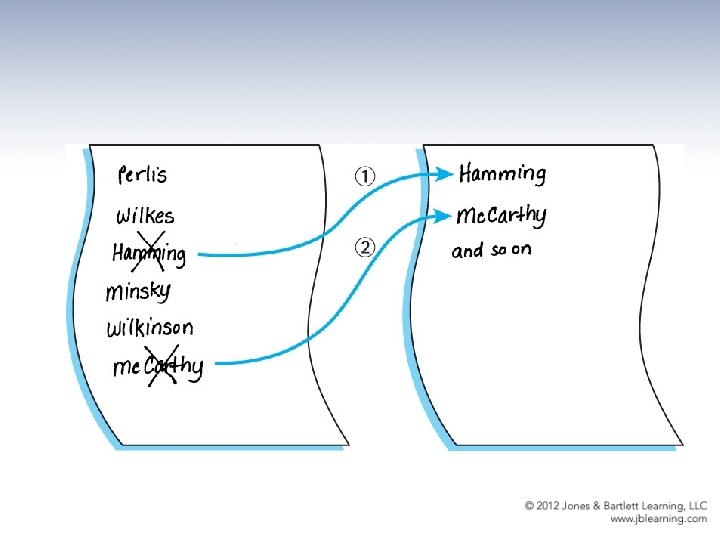
Selection Sort • If we were handed a list of names on a sheet of paper and asked to put them in alphabetical order, we might use this general approach: – Select the name that comes first in alphabetical order, and write it on a second sheet of paper. – Cross the name out on the original sheet. – Repeat steps 1 and 2 for the second name, the third name, and so on until all the names on the original sheet have been crossed out and written onto the second sheet, at which point the list on the second sheet is sorted.

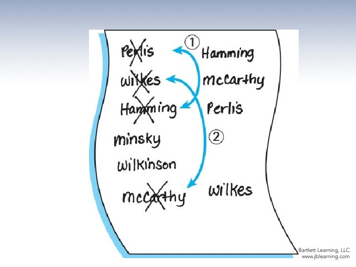
An improvement • Our algorithm is simple but it has one drawback: It requires space to store two complete lists. • Instead of writing the “first” name onto a separate sheet of paper, exchange it with the name in the first location on the original sheet. And so on.

Selection Sort Algorithm Selection. Sort for current going from 0 to SIZE - 2 Find the index in the array of the smallest unsorted element Swap the current element with the smallest unsorted one An example is depicted on the following slide …

Selection Sort Snapshot

Selection Sort Code static int min. Index(int start. Index, int end. Index) // Returns the index of the smallest value in // values[start. Index]. . values[end. Index]. { int index. Of. Min = start. Index; for (int index = start. Index + 1; index <= end. Index; index++) if (values[index] < values[index. Of. Min]) index. Of. Min = index; return index. Of. Min; } static void selection. Sort() // Sorts the values array using the selection sort algorithm. { int end. Index = SIZE – 1; for (int current = 0; current < end. Index; current++) swap(current, min. Index(current, end. Index)); }

Testing Selection Sort The test harness: init. Values(); print. Values(); System. out. println("values is sorted: " + is. Sorted()); System. out. println(); selection. Sort(); System. out. println("Selection Sort calledn"); print. Values(); System. out. println("values is sorted: " + is. Sorted()); System. out. println(); The resultant output: the values array is: 92 66 38 17 21 78 10 43 69 19 17 96 29 19 77 24 47 01 97 91 13 33 84 93 49 85 09 54 13 06 21 21 93 49 67 42 25 29 05 74 96 82 26 25 11 74 03 76 29 10 values is sorted: false Selection Sort called the values array is: 01 03 05 06 09 10 10 11 13 13 17 17 19 19 21 21 21 24 25 25 26 29 29 29 33 38 42 43 47 49 49 54 66 67 69 74 74 76 77 78 82 84 85 91 92 93 93 96 96 97 values is sorted: true

Selection Sort Analysis • We describe the number of comparisons as a function of the number of elements in the array, i. e. , SIZE. To be concise, in this discussion we refer to SIZE as N • The min. Index method is called N - 1 times • Within min. Index, the number of comparisons varies: – in the first call there are N - 1 comparisons – in the next call there are N - 2 comparisons – and so on, until in the last call, when there is only 1 comparison • The total number of comparisons is (N – 1) + (N – 2) + (N – 3) +. . . + 1 = N(N – 1)/2 = 1/2 N 2 – 1/2 N • The Selection Sort algorithm is O(N 2)

Number of Comparisons Required to Sort Arrays of Different Sizes Using Selection Sort Number of Elements 10 20 100 1, 000 10, 000 Number of Comparisons 45 190 4, 950 499, 500 49, 995, 000

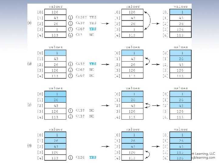
Bubble Sort • With this approach the smaller data values “bubble up” to the front of the array … • Each iteration puts the smallest unsorted element into its correct place, but it also makes changes in the locations of the other elements in the array. • The first iteration puts the smallest element in the array into the first array position: – starting with the last array element, we compare successive pairs of elements, swapping whenever the bottom element of the pair is smaller than the one above it – in this way the smallest element “bubbles up” to the top of the array. • The next iteration puts the smallest element in the unsorted part of the array into the second array position, using the same technique • The rest of the sorting process continues in the same way

Bubble Sort Algorithm Bubble. Sort Set current to the index of first element in the array while more elements in unsorted part of array “Bubble up” the smallest element in the unsorted part, causing intermediate swaps as needed Shrink the unsorted part of the array by incrementing current bubble. Up(start. Index, end. Index) for index going from end. Index DOWNTO start. Index +1 if values[index] < values[index - 1] Swap the value at index with the value at index - 1 An example is depicted on the following slide …

Bubble Sort Snapshot

Bubble Sort Code static void bubble. Up(int start. Index, int end. Index) // Switches adjacent pairs that are out of order // between values[start. Index]. . values[end. Index] // beginning at values[end. Index]. { for (int index = end. Index; index > start. Index; index--) if (values[index] < values[index – 1]) swap(index, index – 1); } static void bubble. Sort() // Sorts the values array using the bubble sort algorithm. { int current = 0; while (current < SIZE – 1) { bubble. Up(current, SIZE – 1); current++; } }

Bubble Sort Analysis • Analyzing the work required by bubble. Sort is the same as for the straight selection sort algorithm. • The comparisons are in bubble. Up, which is called N – 1 times. • There are N – 1 comparisons the first time, N – 2 comparisons the second time, and so on. • Therefore, bubble. Sort and selection. Sort require the same amount of work in terms of the number of comparisons. • The Bubble Sort algorithm is O(N 2)

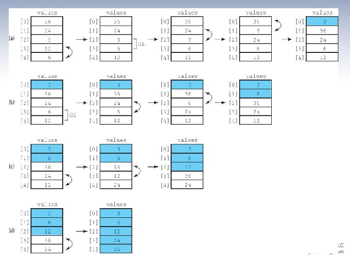
Insertion Sort • In Chapter 6, we created a sorted list by inserting each new element into its appropriate place in an array. Insertion Sort uses the same approach for sorting an array. • Each successive element in the array to be sorted is inserted into its proper place with respect to the other, already sorted elements. • As with the previous sorts, we divide our array into a sorted part and an unsorted part. – Initially, the sorted portion contains only one element: the first element in the array. – Next we take the second element in the array and put it into its correct place in the sorted part; that is, values[0] and values[1] are in order with respect to each other. – Next the value in values[2] is put into its proper place, so values[0]. . values[2] are in order with respect to each other. – This process continues until all the elements have been sorted.

Insertion Sort Algorithm insertion. Sort for count going from 1 through SIZE - 1 insert. Element(0, count) Insert. Element(start. Index, end. Index) Set finished to false Set current to end. Index Set more. To. Search to true while more. To. Search AND NOT finished if values[current] < values[current - 1] swap(values[current], values[current - 1]) Decrement current Set more. To. Search to (current does not equal start. Index) else Set finished to true An example is depicted on the following slide …

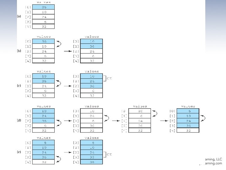
Insertion Sort Snapshot

Insertion Sort Code static void insert. Element(int start. Index, int end. Index) // Upon completion, values[0]. . values[end. Index] are sorted. { boolean finished = false; int current = end. Index; boolean more. To. Search = true; while (more. To. Search && !finished) { if (values[current] < values[current – 1]) { swap(current, current – 1); current--; more. To. Search = (current != start. Index); } else finished = true; } } static void insertion. Sort() // Sorts the values array using the insertion sort algorithm. { for (int count = 1; count < SIZE; count++) insert. Element(0, count); }

Insertion Sort Analysis • The general case for this algorithm mirrors the selection. Sort and the bubble. Sort, so the general case is O(N 2). • But insertion. Sort has a “best” case: The data are already sorted in ascending order – insert. Element is called N times, but only one comparison is made each time and no swaps are necessary. • The maximum number of comparisons is made only when the elements in the array are in reverse order.

10. 3 O(N log 2 N) Sorts • O(N 2) sorts and are very time consuming for sorting large arrays. • Several sorting methods that work better when N is large are presented in this section. • The efficiency of these algorithms is achieved at the expense of the simplicity seen in the straight selection, bubble, and insertion sorts.

The Merge Sort • The sorting algorithms covered in Section 10. 2 are all O(N 2). • Note that N 2 is a lot larger than (1/2 N)2 + (1/2 N)2 = 1/2 N 2 • If we can cut the array into two pieces, sort each segment, and then merge the two back together, we should end up sorting the entire array with a lot less work.

Rationale for Divide and Conquer

Merge Sort Algorithm merge. Sort Cut the array in half Sort the left half Sort the right half Merge the two sorted halves into one sorted array Because merge. Sort is itself a sorting algorithm, we might as well use it to sort the two halves. We can make merge. Sort a recursive method and let it call itself to sort each of the two subarrays: merge. Sort—Recursive Cut the array in half merge. Sort the left half merge. Sort the right half Merge the two sorted halves into one sorted array

Merge Sort Summary Method merge. Sort(first, last) Definition: Sorts the array elements in ascending order. Size: last - first + 1 Base Case: If size less than 2, do nothing. General Case: Cut the array in half. merge. Sort the left half. merge. Sort the right half. Merge the sorted halves into one sorted array.

Strategy for merging two sorted arrays

Our actual merge problem

Our solution

The merge algorithm merge (left. First, left. Last, right. First, right. Last) (uses a local array, temp. Array) Set index to left. First while more elements in left half AND more elements in right half if values[left. First] < values[right. First] Set temp. Array[index] to values[left. First] Increment left. First else Set temp. Array[index] to values[right. First] Increment right. First Increment index Copy any remaining elements from left half to temp. Array Copy any remaining elements from right half to temp. Array Copy the sorted elements from temp. Array back into values

The merge. Sort method The code for merge follows the algorithm on the previous slide. It can be found on page 676 -677 of the textbook. merge does most of the work! Here is merge. Sort: static void merge. Sort(int first, int last) // Sorts the values array using the merge sort algorithm. { if (first < last) { int middle = (first + last) / 2; merge. Sort(first, middle); merge. Sort(middle + 1, last); merge(first, middle + 1, last); } }

Analysing Merge Sort

Analyzing Merge Sort • The total work needed to divide the array in half, over and over again until we reach subarrays of size 1, is O(N). • It takes O(N) total steps to perform merging at each “level” of merging. • The number of levels of merging is equal to the number of times we can split the original array in half – If the original array is size N, we have log 2 N levels. (This is the same as the analysis of the binary search algorithm in Section 6. 6. ) • Because we have log 2 N levels, and we require O(N) steps at each level, the total cost of the merge operation is: O(N log 2 N). • Because the splitting phase was only O(N), we conclude that Merge Sort algorithm is O(N log 2 N).

Comparing N 2 and N log 2 N N 32 64 128 256 512 1024 2048 4096 log 2 N 5 6 7 8 9 10 11 12 N 2 1, 024 4. 096 16, 384 65, 536 262, 144 1, 048, 576 4, 194, 304 16, 777, 216 N log 2 N 160 384 896 2, 048 4, 608 10, 240 22, 528 49, 152

Drawback of Merge Sort • A disadvantage of merge. Sort is that it requires an auxiliary array that is as large as the original array to be sorted. • If the array is large and space is a critical factor, this sort may not be an appropriate choice. • Next we discuss two O(N log 2 N) sorts that move elements around in the original array and do not need an auxiliary array.

Quick Sort • A divide-and-conquer algorithm • Inherently recursive • At each stage the part of the array being sorted is divided into two “piles”, with everything in the left pile less than everything in the right pile • The same approach is used to sort each of the smaller piles (a smaller case). • This process goes on until the small piles do not need to be further divided (the base case).

Quick Sort Summary Method quick. Sort (first, last) Definition: Sorts the elements in sub array values[first]. . values[last]. Size: last - first + 1 Base Case: If size less than 2, do nothing. General Case: Split the array according to splitting value. quick. Sort the elements <= splitting value. quick. Sort the elements > splitting value.

The Quick Sort Algorithm quick. Sort if there is more than one element in values[first]. . values[last] Select split. Val Split the array so that values[first]. . values[split. Point – 1] <= split. Val values[split. Point] = split. Val values[split. Point + 1]. . values[last] > split. Val quick. Sort the left sub array quick. Sort the right sub array The algorithm depends on the selection of a “split value”, called split. Val, that is used to divide the array into two sub arrays. How do we select split. Val? One simple solution is to use the value in values[first] as the splitting value.

Quick Sort Steps

The quick. Sort method static void quick. Sort(int first, int last) { if (first < last) { int split. Point; split. Point = split(first, last); // values[first]. . values[split. Point – 1] <= split. Val // values[split. Point] = split. Val // values[split. Point+1]. . values[last] > split. Val quick. Sort(first, split. Point – 1); quick. Sort(split. Point + 1, last); } }

The split operation The code for split is on page 684

Analyzing Quick Sort • On the first call, every element in the array is compared to the dividing value (the “split value”), so the work done is O(N). • The array is divided into two sub arrays (not necessarily halves) • Each of these pieces is then divided in two, and so on. • If each piece is split approximately in half, there are O(log 2 N) levels of splits. At each level, we make O(N) comparisons. • So Quick Sort is an O(N log 2 N) algorithm.

Drawbacks of Quick Sort • Quick Sort isn’t always quicker. – There are log 2 N levels of splits if each split divides the segment of the array approximately in half. As we’ve seen, the array division of Quick Sort is sensitive to the order of the data, that is, to the choice of the splitting value. – If the splits are very lopsided, and the subsequent recursive calls to quick. Sort also result in lopsided splits, we can end up with a sort that is O(N 2). • What about space requirements? – There can be many levels of recursion “saved” on the system stack at any time. – On average, the algorithm requires O(log 2 N) extra space to hold this information and in the worst case requires O(N) extra space, the same as Merge Sort.

Quick Sort • Despite the drawbacks remember that Quick Sort is VERY quick for large collections of random data

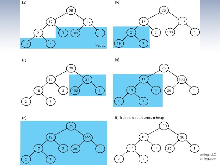
Heap Sort • In Chapter 9, we discussed the heap - because of its order property, the maximum value of a heap is in the root node. • The general approach of the Heap Sort is as follows: – take the root (maximum) element off the heap, and put it into its place. – reheap the remaining elements. (This puts the nextlargest element into the root position. ) – repeat until there are no more elements. • For this to work we must first arrange the original array into a heap

Building a heap build. Heap for index going from first nonleaf node up to the root node reheap. Down(values[index], index) See next slide …

The changing contents of the array

The Sort Nodes algorithm Sort Nodes for index going from last node up to next-to-root node Swap data in root node with values[index] reheap. Down(values[0], 0, index 2 1)

The heap. Sort method static void heap. Sort() // Post: The elements in the array values are sorted by key { int index; // Convert the array of values into a heap for (index = SIZE/2 – 1; index >= 0; index--) reheap. Down(values[index], index, SIZE – 1); // Sort the array for (index = SIZE – 1; index >=1; index--) { swap(0, index); reheap. Down(values[0], 0, index – 1); } }

Analysis of Heap Sort • Consider the sorting loop – it loops through N ─ 1 times, swapping elements and reheaping – the comparisons occur in reheap. Down (actually in its helper method new. Hole) – a complete binary tree with N nodes has O(log 2(N + 1)) levels – in the worst cases, then, if the root element had to be bumped down to a leaf position, the reheap. Down method would make O(log 2 N) comparisons. – so method reheap. Down is O(log 2 N) – multiplying this activity by the N ─ 1 iterations shows that the sorting loop is O(N log 2 N). • Combining the original heap build, which is O(N), and the sorting loop, we can see that Heap Sort requires O(N log 2 N) comparisons.

The Heap Sort • For small arrays, heap. Sort is not very efficient because of all the “overhead. ” • For large arrays, however, heap. Sort is very efficient. • Unlike Quick Sort, Heap Sort’s efficiency is not affected by the initial order of the elements. • Heap Sort is also efficient in terms of space – it only requires constant extra space. • Heap Sort is an elegant, fast, robust, space efficient algorithm!

10. 4 More Sorting Considerations • In this section we wrap up our coverage of sorting by – revisiting testing – revisiting efficiency – discussing special concerns involved with sorting objects rather than primitive types – considering the “stability” of sorting algorithms

Testing • To thoroughly test our sorting methods we should – vary the size of the array – vary the original order of the array • • Random order Reverse order Almost sorted All identical elements

Efficiency • When N is small the simple sorts may be more efficient than the “fast” sorts because they require less overhead. • Sometimes it may be desirable, for efficiency considerations, to streamline the code as much as possible, even at the expense of readability. For instance, instead of using a swap method directly code the swap operation within the sorting method.

Special Concerns when Sorting Objects • When sorting an array of objects we are manipulating references to the object, and not the objects themselves

Using the Comparable Interface • For our sorted lists, binary search trees and priority queues we used objects that implemented Java’s Comparable interface. • The only requirement for a Comparable object is that it provides a compare. To operation. • A limitation of this approach is that a class can only have one compare. To method. What if we have a class of objects, for example student records, that we want to sort in many various ways: by name, by grade, by zip code, in increasing order, in decreasing order? In this case we need to use the next approach.

Using the Comparator Interface • The Java Library provides another interface related to comparing objects called Comparator. • The interface defines two abstract methods: public abstract int compare(T o 1, T o 2); // Returns a negative integer, zero, or a positive integer to // indicate that o 1 is less than, equal to, or greater than o 2 public abstract boolean equals(Object obj); // Returns true if this Object equals obj; false, otherwise

Using the Comparator Interface • If we pass a Comparator object comp to a sorting method as a parameter, the method can use compare to determine the relative order of two objects and base its sort on that relative order. • Passing a different Comparator object results in a different sorting order. • Now, with a single sorting method, we can produce many different sort orders.

Example • To allow us to concentrate on the topic of discussion, we use a simple circle class, with public instance variables: package ch 10. circles; public class Sort. Circle { public int x. Value; public int y. Value; public int radius; public boolean solid; } • Here is the definition of a Comparator object that orders Sort. Circles based on their x. Value: Comparator<Circle> x. Comp = new Comparator<Circle>() { public int compare(Sort. Circle a, Sort. Circle b) { return (a. x. Value – b. x. Value); } };

Example • Here is a selection. Sort method, along with its helper method min. Index, that accepts and uses a Comparator object static int min. Index(int start. Index, int end. Index, Comparator<Sort. Circle> comp) // Returns the index of the smallest value in // values[start. Index]. . values[end. Index]. { int index. Of. Min = start. Index; for (int index = start. Index + 1; index <= end. Index; index++) if (compare(values[index], values[index. Of. Min]) < 0) index. Of. Min = index; return index. Of. Min; } static void selection. Sort(Comparator<Sort. Circle> comp) // Sorts the values array using the selection sort algorithm. { int end. Index = SIZE – 1; for (int current = 0; current < end. Index; current++) swap(current, min. Index(current, end. Index, comp)); }

Stability of a Sorting Algorithm • Stable Sort: A sorting algorithm that preserves the order of duplicates • Of the sorts that we have discussed in this book, only heap. Sort and quick. Sort are inherently unstable

10. 5 Searching • In this section we look at some of the basic “search by value” techniques for lists. • Some of these techniques (linear and binary search) we have seen previously in the text. • In Section 10. 6 we look at an advanced technique, called hashing, that can often provide O(1) searches by value.

Linear Searching • If we want to add elements as quickly as possible to a list, and we are not as concerned about how long it takes to find them we would put the element – into the last slot in an array-based list – into the first slot in a linked list • To search this list for the element with a given key, we must use a simple linear (or sequential) search – Beginning with the first element in the list, we search for the desired element by examining each subsequent element’s key until either the search is successful or the list is exhausted. – Based on the number of comparisons this search is O(N) – In the worst case we have to make N key comparisons. – On the average, assuming that there is an equal probability of searching for any element in the list, we make N/2 comparisons for a successful search

High-Probability Ordering • Sometimes certain list elements are in much greater demand than others. We can then improve the search: – Put the most-often-desired elements at the beginning of the list – Using this scheme, we are more likely to make a hit in the first few tries, and rarely do we have to search the whole list. • If the elements in the list are not static or if we cannot predict their relative demand, we can – move each element accessed to the front of the list – as an element is found, it is swapped with the element that precedes it • Lists in which the relative positions of the elements are changed in an attempt to improve search efficiency are called self-organizing or self-adjusting lists.

Sorted Lists • If the list is sorted, a sequential search no longer needs to search the whole list to discover that an element does not exist. It only needs to search until it has passed the element’s logical place in the list—that is, until an element with a larger key value is encountered. • Another advantage of linear searching is its simplicity. • The binary search is usually faster, however, it is not guaranteed to be faster for searching very small lists. • As the number of elements increases, however, the disparity between the linear search and the binary search grows very quickly. • The binary search is appropriate only for list elements stored in a sequential array-based representation. • However, the binary search tree allows us to perform a binary search on a linked data representation

10. 6 Hashing

Definitions • Hash Functions: A function used to manipulate the key of an element in a list to identify its location in the list • Hashing: The technique for ordering and accessing elements in a list in a relatively constant amount of time by manipulating the key to identify its location in the list • Hash table: Term used to describe the data structure used to store and retrieve elements using hashing

Our Hashable interface public interface Hashable // Objects of classes that implement this interface can be used // with lists based on hashing. { // A mathematical function used to manipulate the key of an element // in a list to identify its location in the list. int hash(); }

Using the hash method public void add (Hashable element) // Adds element to this list at position element. hash(). { int location; location = element. hash(); list[location] = element; num. Elements++; } public Hashable get(Hashable element) // Returns an element e from this list such // that e. equals(element). { int location; location = element. hash(); return (Hashable)list[location]; }

Collisions • Collision: The condition resulting when two or more keys produce the same hash location • Linear probing: Resolving a hash collision by sequentially searching a has table beginning at the location returned by the hash function

Revised methods public static void add (Hashable element) // Adds element to this list at position element. hash(), // or the next free array slot. { int location; location = element. hash(); while (list[location] != null) location = (location + 1) % list. length; list[location] = element; num. Elements++; } public static Hashable get(Hashable element) // Returns an element e from this list such that e. equals(element). { int location; location = element. hash(); while (!list[location]. equals(element)) location = (location + 1) % list. length; return (Hashable)list[location]; }

Handling collisions with linear probing

Removing an element • An approach could be remove (element) Set location to element. hash( ) Set list[location] to null • Collisions, however, complicate the matter. We cannot be sure that our element is in location element. hash(). • We must examine every array element, starting with location element. hash(), until we find the matching element. • We cannot stop looking when we reach an empty location, because that location may represent an element that was previously removed. • This problem illustrates that hash tables, in the forms that we have studied thus far, are not the most effective data structure for implementing lists whose elements may be deleted.

More Considerations • Clustering: The tendency of elements to become unevenly distributed in the hash table, with many elements clustering around a single hash location • Rehashing: Resolving a collision by computing a new hash location from a hash function that manipulates the original location rather than the element’s key • Quadratic probing Resolving a hash collision by using the rehashing formula (Hash. Value +/- I 2) % array-size • Random probing Resolving a hash collision by generating pseudo-random hash values in successive applications of the rehash function

Buckets and Chaining • Bucket A collection of elements associated with a particular hash location • Chain A linked list of elements that share the same hash location

Handling collisions by hashing with buckets

Handling collisions by hashing with chaining

Java’s Support for Hashing • The Java Library includes a Hash. Table class that uses hash techniques to support storing objects in a table. • The library includes several other collection classes, such as Hash. Set, that provide an ADT whose underlying implementation uses the approaches described in this section. • The Java Object class exports a hash. Code method that returns an int hash code. Therefore all Java objects have an associated hash code. – The standard Java hash code for an object is a function of the object’s memory location. • For most applications, hash codes based on memory locations are not usable. Therefore, many of the Java classes that define commonly used objects (such as String and Integer), override the Object class’s hash. Code method with one that is based on the contents of the object. • If you plan to use hash tables in your programs, you should do likewise.