Discrete Cosine Transform and Image Compression Biswapati Jana

Common Applications l JPEG Format l MPEG-1 and MPEG-2 l MP 3, Advanced Audio Coding etc. l What’s l in common? All share, in some form or another, a DCT method for compression.

Overview l One-dimensional DCT l Two-dimensional DCT l Image Compression (grayscale)

One-dimensional DCT Definition: Let n be a positive integer. The one-dimensional DCT of order n is defined by an n x n matrix C whose entries are

The Advantage of Orthogonality C orthogonal: CTC = I l Implies C-1 = CT l l Makes solving matrix equations easy Solve Y = CXCT for any X: l CTY = CTCXCT = XCT l CTYC = XCTC = X l

One-dimensional DCT The discrete cosine transform, C, has one basic characteristic: it is a real orthogonal matrix.

One-dimensional DCT Suppose we are given a vector The Discrete Cosine Transform of x is the ndimensional vector Where C is defined as

Two-Dimensional DCT Use One-Dimensional DCT in both horizontal and vertical directions. First direction F = C*XT Second direction G = C*FT We can say 2 D-DCT is the matrix: Y = C(CXT)T

DCT l The Discrete Cosine Transform (DCT) is used for JPEG images to transform them into frequencies. l DCT is a mathematical transform (typically a cosine function) that converts the pixels by seemingly ’spreading’ the location of the pixel values over part of the image.

DCT l It does this by grouping the pixels into 8 x 8 blocks and transforming them from 64 values into 64 frequencies (DCT coefficients). By modifying just a single DCT coefficient, the entire 64 pixels in that block will be affected.

DCT l The image on the right is the result after applying DCT to the block of the image.

DCT l Note, how the largest value is located in the top-left corner of the block, this is the actually the lowest frequency. l The value is so high because the data is encoded with the highest importance and the lowest frequency. l This, in simpler terms means that this value is the average value of all the pixel values in this block

DCT l The values are typically always high around the top-left corner of a DCT block but note that the numbers closest to zero seem to populate around the lower-right corner of the block. l These are the high frequencies and it is these values that are removed during the next step.

Image Compression Image compression is a method that reduces the amount of memory it takes to store in image. l We will exploit the fact that the DCT matrix is based on our visual system for the purpose of image compression. l This means we can delete the least significant values without our eyes noticing the difference. l

Image Compression l Now we have found the matrix Y = C(CXT)T l Using the DCT, the entries in Y will be organized based on the human visual system. l The most important values to our eyes will be placed in the upper left corner of the matrix. l The least important values will be mostly in the lower right corner of the matrix. Most Important Semi. Important Least Important

Image Compression 8 x 8 Pixels Image

Image Compression l Gray-Scale Example: l Value Range 0 (black) --- 255 (white) 63 33 36 28 63 81 27 18 17 11 22 48 72 52 28 15 17 16 132 100 56 19 10 9 187 186 166 88 13 34 184 203 199 177 82 44 211 214 208 198 134 52 211 210 203 191 133 79 X 86 98 104 108 47 77 21 55 43 51 97 73 78 83 74 86

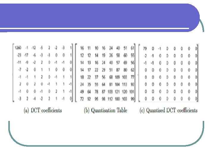
Image Compression l 2 D-DCT of matrix Numbers are coefficients of polynomial -304 210 -327 -260 93 -84 89 33 -9 42 -5 15 10 3 12 30 104 -69 10 67 70 -10 -66 16 24 -19 -20 -26 18 27 -7 -10 17 32 -1 2 0 -3 -3 Y 20 -15 -2 21 -17 -15 3 -6 -12 7 21 8 -5 9 -3 0 29 -7 -4 7 -2 -3 12 -1

Image Compression l Cut -304 210 -327 -260 93 -84 89 33 -9 42 -5 15 10 0 the least significant components 104 -69 10 67 70 -10 -66 16 24 -19 -20 0 18 0 0 0 20 -12 0 -15 0 0 0 0 0 As you can see, we save a little over half the original memory.

Inverse 2 D-DCT gives us Y = C(CXT)T which can be rewritten Y = CXCT Since C is an orthogonal we can solve for X using the fact C-1 = CT Therefore, X = CTYC

Reconstructing the Image l In Mathematical terms: l Let X = (xij) be a matrix of n 2 real numbers Y = (ykl) be the 2 D-DCT of X a 0 = 1/sqrt(2) and ak = 1 for k > 0 l Then: l l Satisfies Pn(I, j) = xij for I, j=0, …, n-1

Reconstructing the Image l New Matrix and Compressed Image 55 41 27 39 56 69 92 106 35 22 7 16 35 59 88 101 65 49 21 5 6 28 62 73 130 114 75 28 -7 -1 33 46 180 175 148 95 33 16 45 59 200 206 203 165 92 55 71 82 205 207 214 193 121 70 75 83 214 205 209 196 129 75 78 85

Can You Tell the Difference? Original Compressed

Image Compression Original Compressed

Linear Quantization We will not zero the bottom half of the matrix. l The idea is to assign fewer bits of memory to store information in the lower right corner of the DCT matrix. l Quantisation is the process of taking the remaining coefficients and dividing them individually against a predetermined set of values and then rounding the results to the nearest real number value. l

Linear Quantization l The higher these pre-determined values are determines how much detail will be removed from the image. The higher the numbers, the more detail is eliminated. l The goal is to eliminate the high frequency (lower-right) values. l There are only a few values that hold numbers other than zero - the majority will always be zeros.

Imagine you have a birds-eye view on a dense collection of trees. There may be smaller trees that are situated underneath the trees that you can see, but as you cannot see them, it would not affect your view whether they were there or not. l This is exactly the same principle for quantisation – by eliminating the values that would not make a difference to the image should they not exist, a great deal of data can be removed with minimum effect on the quality. l

Linear Quantization Use Quantization Matrix (Q) qkl = 8 p(k + l + 1) for 0 < k, l < 7 Q=p* 8 16 24 32 40 48 56 64 72 80 88 40 48 56 64 72 80 88 72 80 88 96 104 88 95 104 112 96 104 112 120

Linear Quantization l p is called the loss parameter l It acts like a “knob” to control compression l The greater p is the more you compress the image

Linear Quantization We divide the each entry in the DCT matrix by the Quantization Matrix -304 210 -327 -260 93 -84 89 33 -9 42 -5 15 10 3 12 30 104 -69 10 67 70 -10 -66 16 24 -19 -20 -26 18 27 -7 -10 17 32 -1 2 0 -3 -3 20 -15 -2 21 -17 -15 3 -6 -12 7 21 8 -5 9 -3 0 29 -7 -4 7 -2 -3 12 -1 8 16 24 32 40 48 56 64 72 80 88 40 48 56 64 72 80 88 72 80 88 96 104 88 95 104 112 96 104 112 120

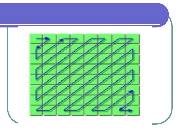
l It is also typical to see the non-zero numbers in the upper left, and zeros as you get towards the lower-right corner. l As this is the case, this stage of JPEG compression reorders the values using a ’zig-zag’ type motion so that similar frequencies are grouped together.

Linear Quantization p=1 -38 13 4 -2 -20 -11 2 2 4 -3 -2 0 3 1 0 0 0 0 0 0 0 0 0 p=4 0 0 0 0 New Y: 14 terms -9 3 1 -1 0 0 -5 -3 1 0 0 0 1 -1 0 0 0 0 0 0 0 0 0 0 0 0 0 0 New Y: 10 terms

Linear Quantization p=1 p=4

Memory Storage l The original image uses one byte (8 bits) for each pixel. Therefore, the amount of memory needed for each 8 x 8 block is: l 8 x (82) = 512 bits

Is This Worth the Work? l The question that arises is “How much memory does this save? ” Linear Quantization p Total bits Bits/pixel X 512 8 1 249 3. 89 2 191 2. 98 3 147 2. 30

The End Thanks for Coming!