DECISION TREE DECISION TREE DATASET no no yes

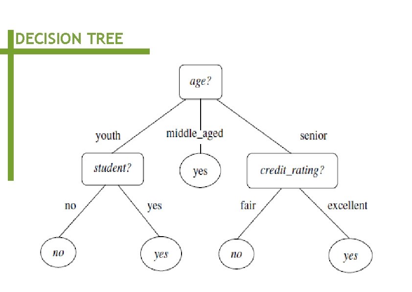
DECISION TREE

DECISION TREE

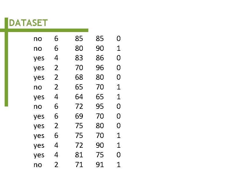
DATASET no no yes yes yes no 6 6 4 2 2 2 4 6 6 2 6 4 4 2 85 80 83 70 68 65 64 72 69 75 75 72 81 71 85 90 86 96 80 70 65 95 70 80 70 90 75 91 0 0 0 1 1 0 1

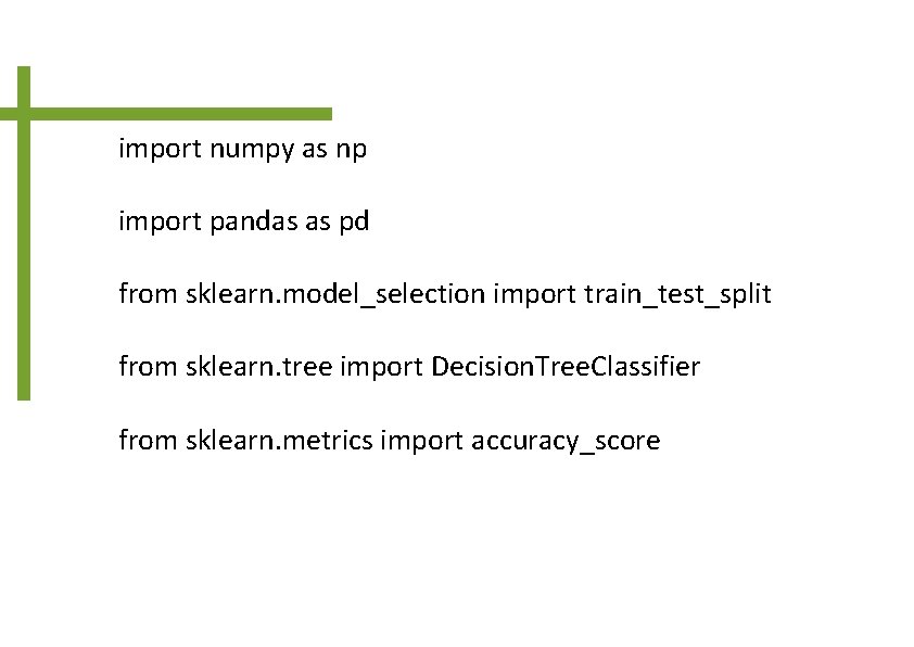
import numpy as np import pandas as pd from sklearn. model_selection import train_test_split from sklearn. tree import Decision. Tree. Classifier from sklearn. metrics import accuracy_score

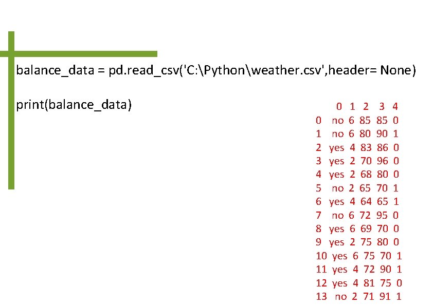
balance_data = pd. read_csv('C: Pythonweather. csv', header= None) print(balance_data) 0 1 2 3 4 0 no 6 85 85 0 1 no 6 80 90 1 2 yes 4 83 86 0 3 yes 2 70 96 0 4 yes 2 68 80 0 5 no 2 65 70 1 6 yes 4 64 65 1 7 no 6 72 95 0 8 yes 6 69 70 0 9 yes 2 75 80 0 10 yes 6 75 70 1 11 yes 4 72 90 1 12 yes 4 81 75 0 13 no 2 71 91 1

print("Dataset Lenght: : ", len(balance_data)) print("Dataset Shape: : ", balance_data. shape) Dataset Lenght: : 14 Dataset Shape: : (14, 5)

X = balance_data. values[: , 1: 5] Y = balance_data. values[: , 0] print (X, Y) [[6 85 85 0] [6 80 90 1] [4 83 86 0] [2 70 96 0] [2 68 80 0] [2 65 70 1] [4 64 65 1] [6 72 95 0] [6 69 70 0] [2 75 80 0] [6 75 70 1] [4 72 90 1] [4 81 75 0] [2 71 91 1]] ['no' 'yes' 'yes' 'yes' 'no']

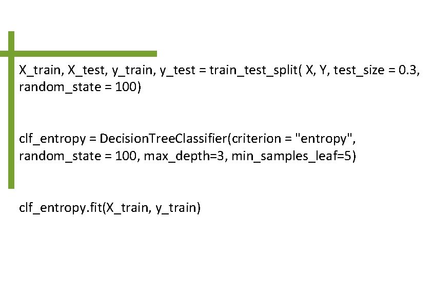
X_train, X_test, y_train, y_test = train_test_split( X, Y, test_size = 0. 3, random_state = 100) clf_entropy = Decision. Tree. Classifier(criterion = "entropy", random_state = 100, max_depth=3, min_samples_leaf=5) clf_entropy. fit(X_train, y_train)

y_pred = clf_entropy. predict(X_test) print(y_pred) ['yes' 'yes']

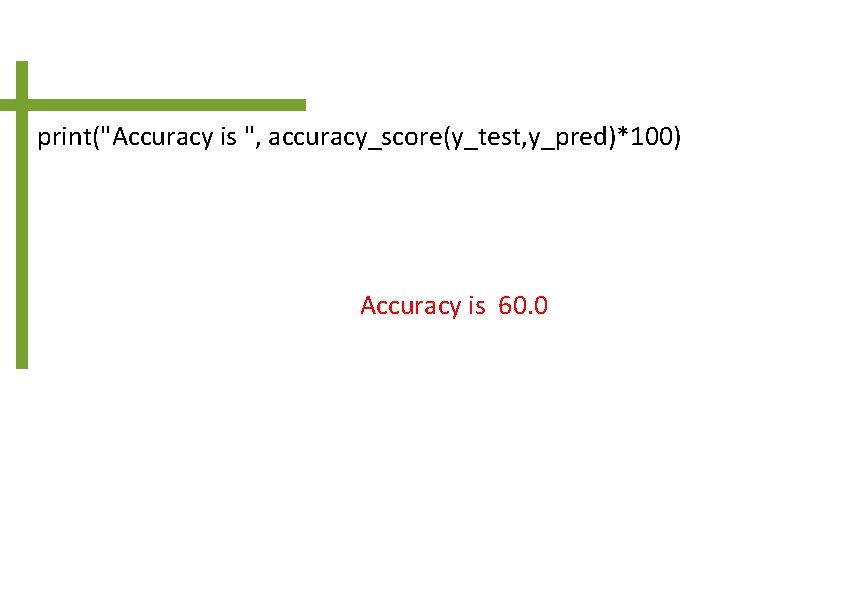
print("Accuracy is ", accuracy_score(y_test, y_pred)*100) Accuracy is 60. 0

print(clf_entropy. predict([[6, 75, 70, 1]])) ['yes']

Naïve Bayes classifier

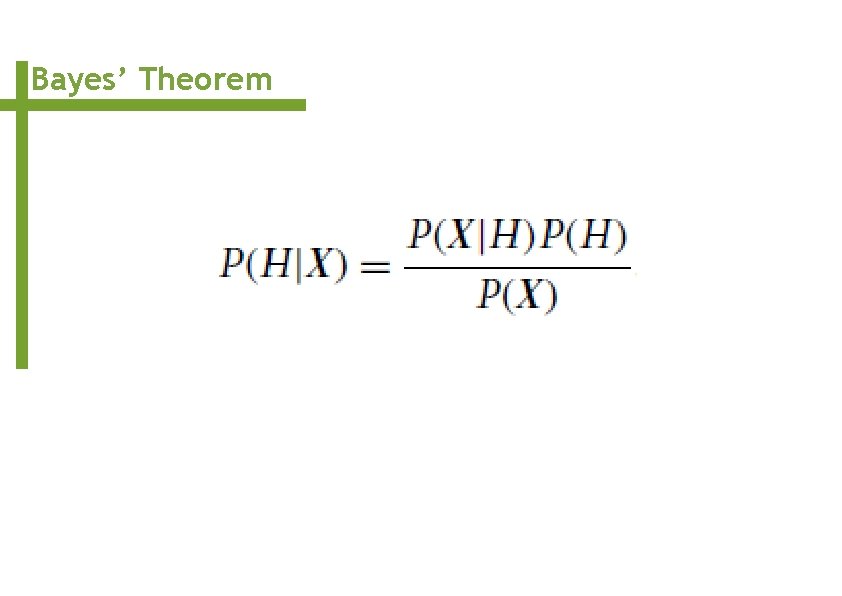
Bayes’ Theorem

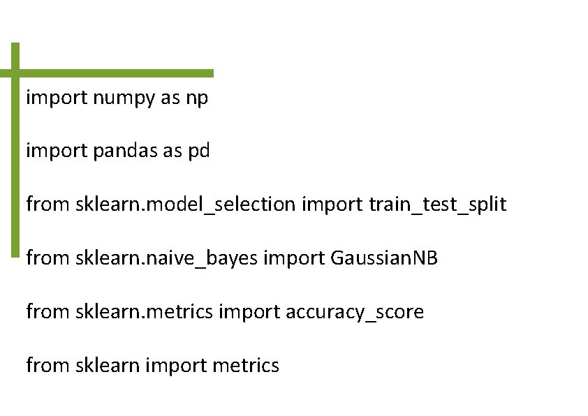
import numpy as np import pandas as pd from sklearn. model_selection import train_test_split from sklearn. naive_bayes import Gaussian. NB from sklearn. metrics import accuracy_score from sklearn import metrics

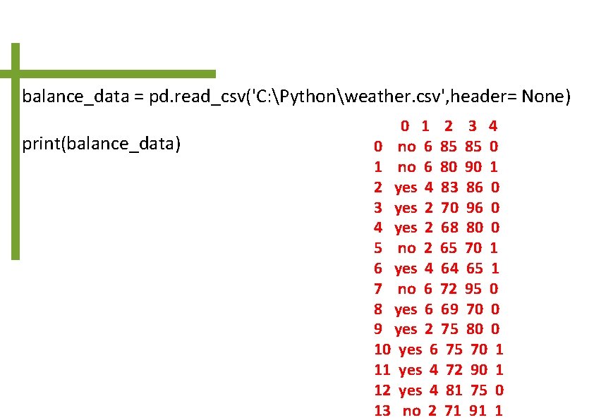
balance_data = pd. read_csv('C: Pythonweather. csv', header= None) print(balance_data) 0 1 2 3 4 0 no 6 85 85 0 1 no 6 80 90 1 2 yes 4 83 86 0 3 yes 2 70 96 0 4 yes 2 68 80 0 5 no 2 65 70 1 6 yes 4 64 65 1 7 no 6 72 95 0 8 yes 6 69 70 0 9 yes 2 75 80 0 10 yes 6 75 70 1 11 yes 4 72 90 1 12 yes 4 81 75 0 13 no 2 71 91 1

balance_data = pd. read_csv('C: Pythonweather. csv', header= None) print(balance_data) 0 1 2 3 4 0 no 6 85 85 0 1 no 6 80 90 1 2 yes 4 83 86 0 3 yes 2 70 96 0 4 yes 2 68 80 0 5 no 2 65 70 1 6 yes 4 64 65 1 7 no 6 72 95 0 8 yes 6 69 70 0 9 yes 2 75 80 0 10 yes 6 75 70 1 11 yes 4 72 90 1 12 yes 4 81 75 0 13 no 2 71 91 1

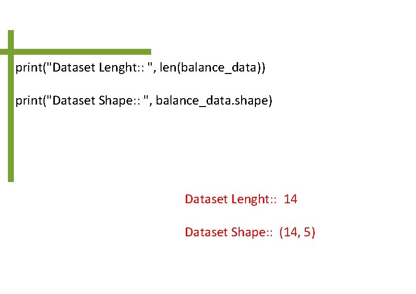
print("Dataset Lenght: : ", len(balance_data)) print("Dataset Shape: : ", balance_data. shape) Dataset Lenght: : 14 Dataset Shape: : (14, 5)

X = balance_data. values[: , 1: 5] Y = balance_data. values[: , 0] print (X, Y) [[6 85 85 0] [6 80 90 1] [4 83 86 0] [2 70 96 0] [2 68 80 0] [2 65 70 1] [4 64 65 1] [6 72 95 0] [6 69 70 0] [2 75 80 0] [6 75 70 1] [4 72 90 1] [4 81 75 0] [2 71 91 1]] ['no' 'yes' 'yes' 'yes' 'no']

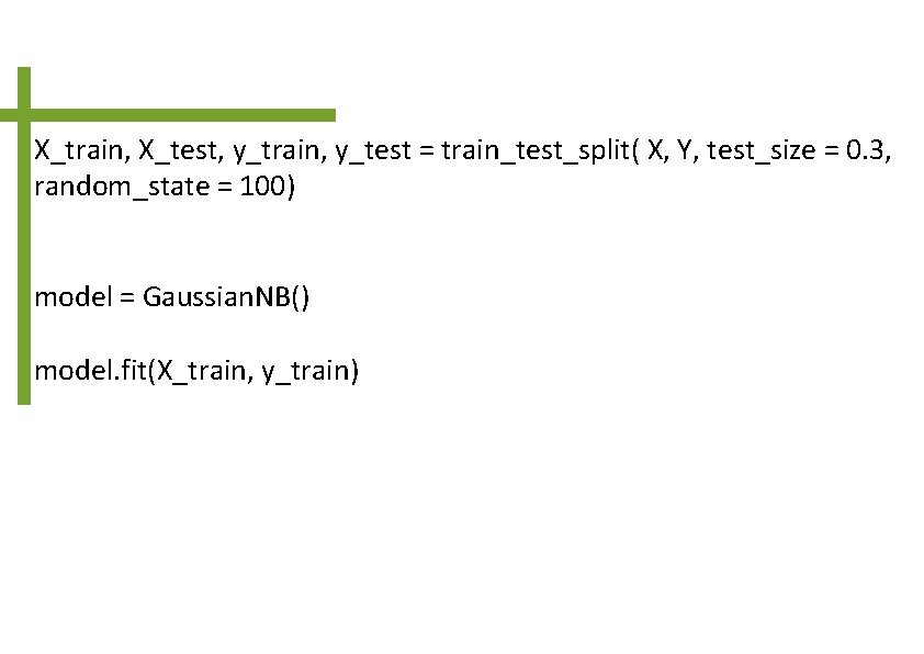
X_train, X_test, y_train, y_test = train_test_split( X, Y, test_size = 0. 3, random_state = 100) model = Gaussian. NB() model. fit(X_train, y_train)

y_pred = model. predict(X_test) print(y_pred) ['no' 'yes']

print(model. predict([[2, 71, 91, 1]])) ['no']

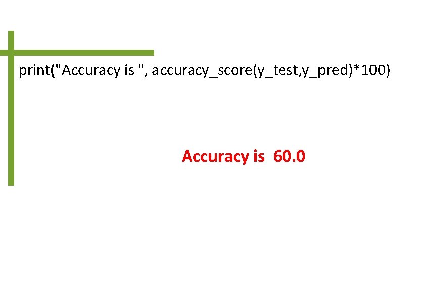
print("Accuracy is ", accuracy_score(y_test, y_pred)*100) Accuracy is 60. 0

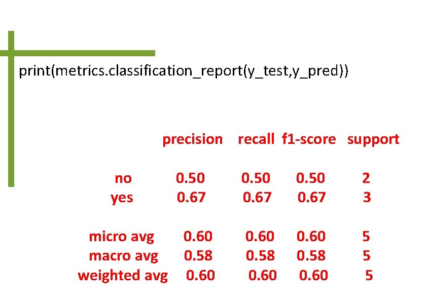
print(metrics. classification_report(y_test, y_pred)) precision recall f 1 -score support no yes 0. 50 0. 67 micro avg 0. 60 macro avg 0. 58 weighted avg 0. 60 0. 50 0. 67 2 3 0. 60 0. 58 0. 60 5 5 5

print(metrics. confusion_matrix(y_test, y_pred)) [[1 1] [1 2]]

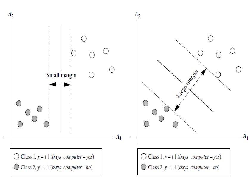
SVM (SUPPORT VECTOR MACHINE)

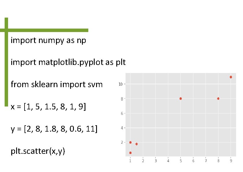
import numpy as np import matplotlib. pyplot as plt from sklearn import svm x = [1, 5, 1. 5, 8, 1, 9] y = [2, 8, 1. 8, 8, 0. 6, 11] plt. scatter(x, y)

X = np. array([[1, 2], [5, 8], [1. 5, 1. 8], [8, 8], [1, 0. 6], [9, 11]]) y = [0, 1, 0, 1] clf = svm. SVC(kernel='linear') clf. fit(X, y)

print(clf. predict([[0. 58, 0. 76]])) [0] print(clf. predict([[10. 58, 10. 76]])) [1]

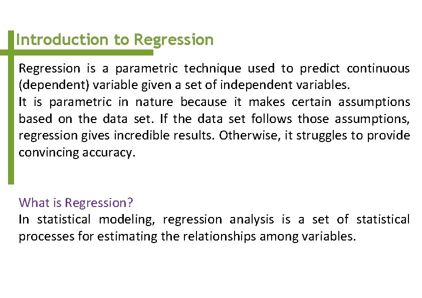
Introduction to Regression is a parametric technique used to predict continuous (dependent) variable given a set of independent variables. It is parametric in nature because it makes certain assumptions based on the data set. If the data set follows those assumptions, regression gives incredible results. Otherwise, it struggles to provide convincing accuracy. What is Regression? In statistical modeling, regression analysis is a set of statistical processes for estimating the relationships among variables.

Regression model Ø Relation between variables where changes in some variables may “explain” or possibly “cause” changes in other variables. Ø Explanatory variables are termed as independent variables and the variables to be explained are termed as dependent variables. Ø Regression model estimates the nature of the relationship between the independent and dependent variables.

Examples Ø Dependent variable is retail price of gasoline in Regina – independent variable is the price of crude oil. Ø Dependent variable is employment income – independent variables might be hours of work, education, occupation, gender, age, region, years of experience, unionization status, etc. Ø Price of a product and quantity produced or sold: Ø Quantity sold affected by price. Dependent variable is quantity of product sold – independent variable is price. Ø Price affected by quantity offered for sale. Dependent variable is price – independent variable is quantity sold.

Uses of regression Ø Amount of change in a dependent variable that results from changes in the independent variable(s) – can be used to estimate elasticities, returns on investment in human capital, etc. Ø Prediction and forecasting of sales, economic growth, etc. Ø Support or negate theoretical model. Ø Modify and improve theoretical models and explanations of phenomena.

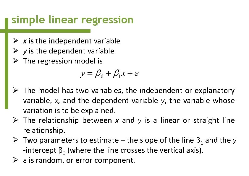
simple linear regression Ø x is the independent variable Ø y is the dependent variable Ø The regression model is Ø The model has two variables, the independent or explanatory variable, x, and the dependent variable y, the variable whose variation is to be explained. Ø The relationship between x and y is a linear or straight line relationship. Ø Two parameters to estimate – the slope of the line β 1 and the y -intercept β 0 (where the line crosses the vertical axis). Ø ε is random, or error component.

Linear Regression

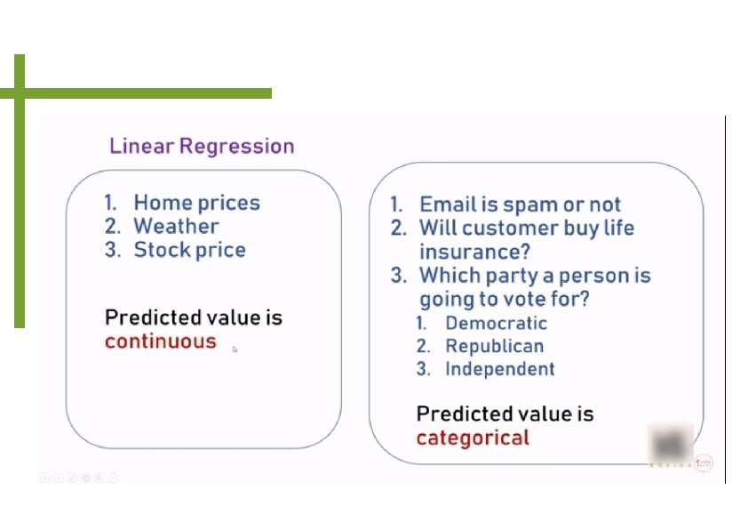
Linear Regression is a machine learning algorithm based on supervised learning. It performs a regression task. Regression, models a target prediction value based on independent variables. It is mostly used for finding out the relationship between variables and forecasting. Different regression models differ based on – the kind of relationship between dependent and independent variables, they are considering and the number of independent variables being used.

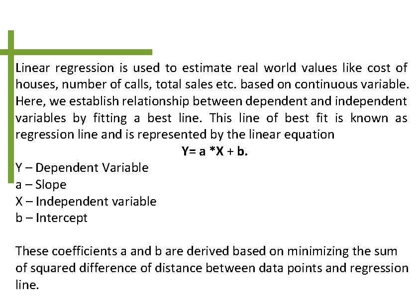
Linear regression is used to estimate real world values like cost of houses, number of calls, total sales etc. based on continuous variable. Here, we establish relationship between dependent and independent variables by fitting a best line. This line of best fit is known as regression line and is represented by the linear equation Y= a *X + b. Y – Dependent Variable a – Slope X – Independent variable b – Intercept These coefficients a and b are derived based on minimizing the sum of squared difference of distance between data points and regression line.

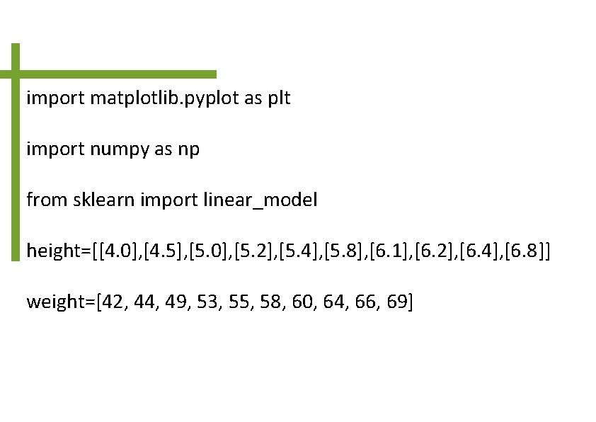
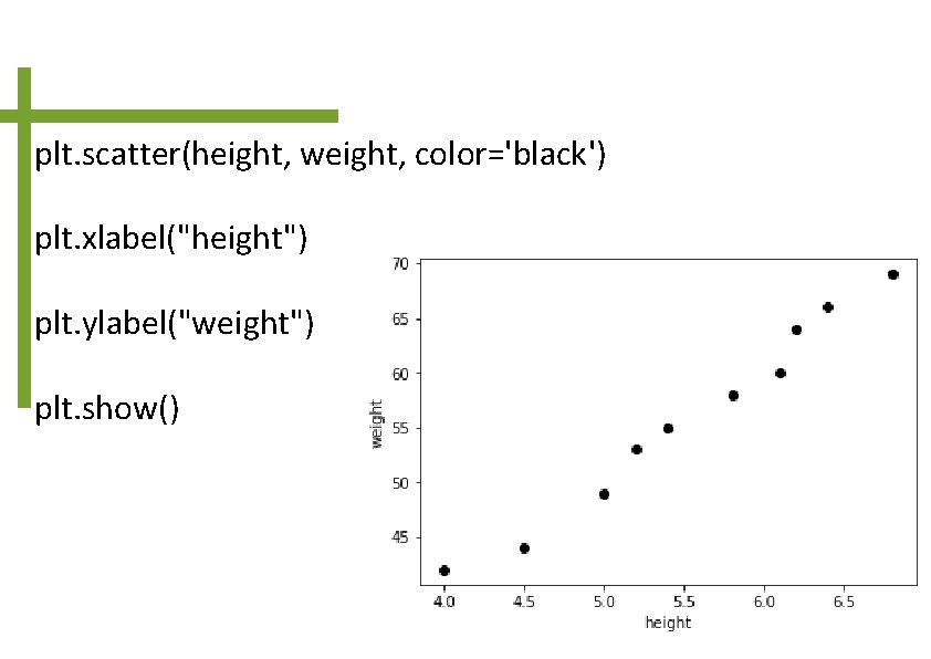
import matplotlib. pyplot as plt import numpy as np from sklearn import linear_model height=[[4. 0], [4. 5], [5. 0], [5. 2], [5. 4], [5. 8], [6. 1], [6. 2], [6. 4], [6. 8]] weight=[42, 44, 49, 53, 55, 58, 60, 64, 66, 69]

plt. scatter(height, weight, color='black') plt. xlabel("height") plt. ylabel("weight") plt. show()

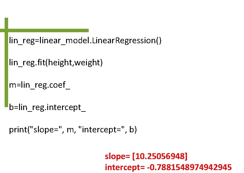
lin_reg=linear_model. Linear. Regression() lin_reg. fit(height, weight) m=lin_reg. coef_ b=lin_reg. intercept_ print("slope=", m, "intercept=", b) slope= [10. 25056948] intercept= -0. 7881548974942945

pred_values=[lin_reg. coef_ * i + lin_reg. intercept_ for i in height] plt. xlabel("height") plt. ylabel("weight") plt. plot(height, pred_values, 'b')

w 1=lin_reg. predict(np. array([[10. 2]])) print("the weight is", w 1) the weight is [103. 76765376]

Logistic Regression

Logistic regression • Logistic regression is another technique borrowed by machine learning from statistics. It is the preferred method for binary classification problems, that is, problems with two class values. • It is a classification algorithm and not a regression algorithm as the name says. It is used to estimate discrete values or values like 0/1, Y/N, T/F based on the given set of independent variable. It predicts the probability of occurrence of an event by fitting data to a logit function. Hence, it is also called logit regression. Since, it predicts the probability, its output values lie between 0 and 1. • Note that taking a log is one of the best mathematical way to replicate a step function.

The following points may be note-worthy when working on logistic regression 1. It is similar to regression in that the objective is to find the values for the coefficients that weigh each input variable. 2. Unlike in linear regression, the prediction for the output is found using a non-linear function called the logistic function. 3. The logistic function appears like a big ‘S’ and will change any value into the range 0 to 1. This is useful because we can apply a rule to the output of the logistic function to assign values to 0 and 1 and predict a class value. 4. The way the logistic regression model is learned, the predictions made by it can also be used as the probability of a given data instance belonging to class 0 or class 1. This can be useful for problems where you need to give more reasoning for a prediction. 5. Like linear regression, logistic regression works better when unrelated attributes of o/p variable is removed and similar attributes are removed.

PYTHON CODE FOR LIGISTIC REGRESSION import pandas as pd import matplotlib. pyplot as plt from sklearn. model_selection import train_test_split from sklearn. linear_model import Logistic. Regression

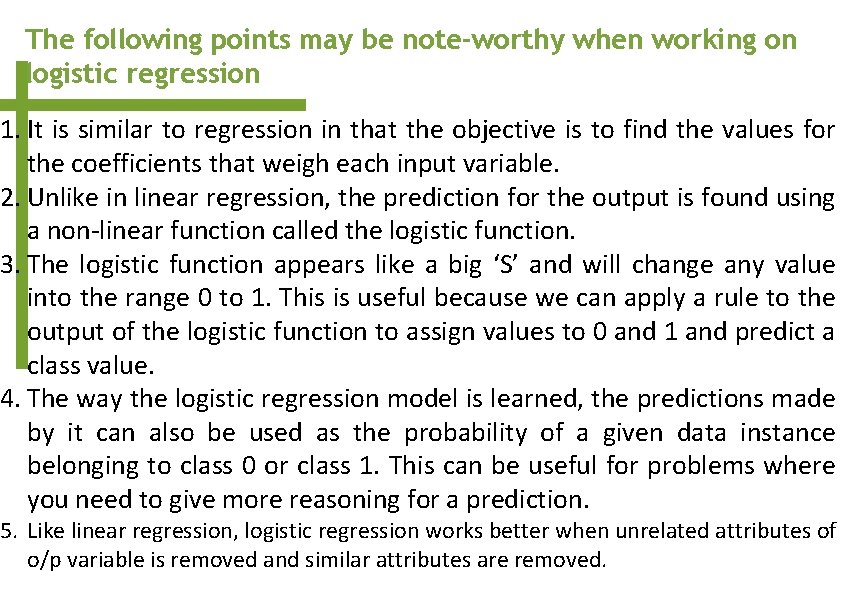
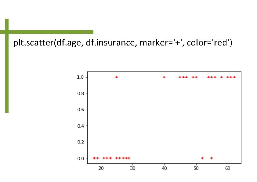
df = pd. read_csv('C: Pythoninsurance_data. csv') print(df) age insurance 0 22 0 1 25 0 2 47 1 3 52 0 4 46 1 5 56 1 6 55 0 7 60 1 8 62 1 9 61 1 10 18 0 11 28 0 12 27 0 13 29 0 14 49 1 15 55 1 16 25 1 17 58 1 18 19 0 19 18 0 20 21 26 0 22 40 1 23 45 1 24 50 1 25 54 1 26 23 0

plt. scatter(df. age, df. insurance, marker='+', color='red')

X_train, X_test, y_train, y_test = train_test_split( df[['age']], df. insurance, test_size=0. 1) model=Logistic. Regression() model. fit(X_train, y_train) m 1=model. predict(X_test) print(m 1) [1 1 0]

m 2=model. predict([[35]]) print(m 2) [1]