ModuleII Decision Tree Learning Introduction Introduction Decision tree

Module-II Decision Tree Learning

Introduction

Introduction • Decision tree learning is a method for approximating discrete- valued target functions, in which the learned function is represented by a decision tree. • Learned trees can also be re-represented as sets of if-then rules to improve human readability. • Most popular of inductive inference algorithms • Have been successfully applied to a broad range of tasks from learning to diagnose medical cases to learning to assess credit risk of loan applicants.

Decision tree representation

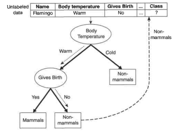
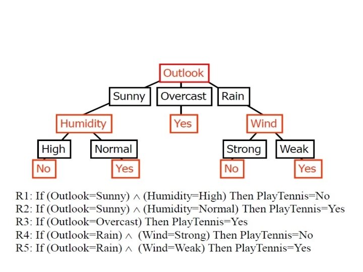
• In general, decision trees represent a disjunction of conjunctions of constraints on the attribute values of instances. • Each path from the tree root to a leaf corresponds to a conjunction of attribute tests, and the tree itself to a disjunction of these conjunctions. For example, the decision tree shown in Figure corresponds to the expression (Outlook = Sunny Λ Humidity = Normal) V (Outlook = Overcast) V (Outlook = Rain Λ Wind = Weak)

APPROPRIATE PROBLEMS FOR DECISION TREE LEARNING decision tree learning is generally best suited to problems with the following characteristics • Instances are represented by attribute-value pairs • The target function has discrete output values • Disjunctive descriptions may be required • The training data may contain errors • The training data may contain missing attribute values Examples : Learning to classify medical patients by their disease, equipment malfunctions by their cause, and loan applicants by their likelihood of defaulting on payments. • Such problems, in which the task is to classify examples into one of a discrete set of possible categories, are often referred to as classification problems.

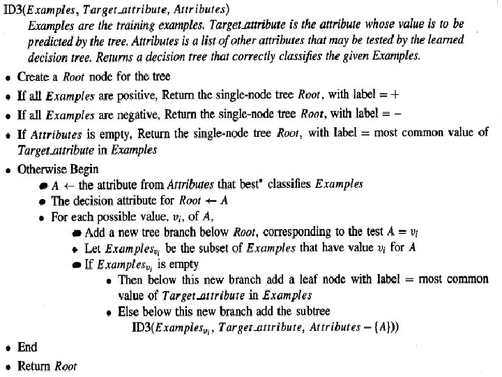
THE BASIC DECISION TREE LEARNING ALGORITHM The core algorithm that employs a top-down, greedy search through the space of possible decision trees. This approach is demonstrated by the ID 3 algorithm (Iterative Dichotomiser 3) In real time we use variations of ID 3 basic algorithm, learns decision trees by constructing them top-down, beginning with the question "which attribute should be tested at the root of the tree? ” The best attribute is selected based on the statistical test at the root node of the tree.

Inventor John Ross Quinlan He is a computer science researcher in data mining and decision theory. He has contributed extensively to the development of decision tree algorithms, including inventing the ID 3 & canonical C 4. 5 algorithms.

Which Attribute Is the Best Classifier? • The central choice in the ID 3 algorithm is selecting which attribute to test at each node in the tree. • We would like to select the attribute that is most useful for classifying examples. • What is a good quantitative measure of the worth of an attribute? We will define a statistical property, called information gain, that measures how well a given attribute separates the training examples according to their target classification. ID 3 uses this information gain measure to select among the candidate attributes at each step while growing the tree.

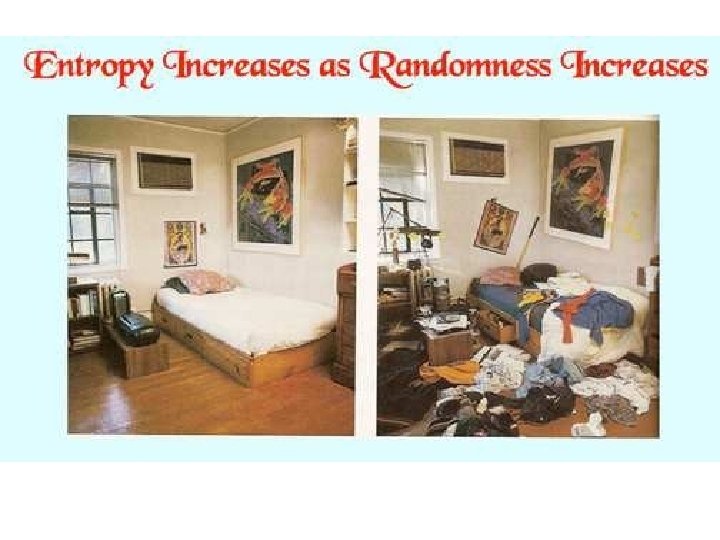
ENTROPY MEASURES HOMOGENEITY OF EXAMPLES • In order to define information gain precisely, we begin by defining a measure commonly used in information theory, called entropy, that characterizes the (im)purity of an arbitrary collection of examples. • Given a collection S, containing positive and negative examples of some target concept, the entropy of S relative to this Boolean classification is • where p⨁, is the proportion of positive examples in S and pΘ, is the proportion of negative examples in S. In all calculations involving entropy we define 0 log 0 to be 0.

• To illustrate, suppose S is a collection of 14 examples of some boolean concept, including 9 positive and 5 negative examples (we adopt the notation [9+, 5 -] to summarize such a sample of data). Then the entropy of S relative to this boolean classification is • Notice that the entropy is 0 if all members of S belong to the same class. For example, if all members are positive (p⨁ = 1), then pΘ, is 0, and Entropy(S) = -1. log 2(1) - 0. log 20 = -1. 0 - 0. log 20 = 0. • Note the entropy is 1 when the collection contains an equal number of positive and negative examples.

• If the collection contains unequal numbers of positive and negative examples, the entropy is between 0 and 1. • Figure shows the form of the entropy function relative to a boolean classification, as p⨁, The entropy function relative to a boolean varies between 0 and 1. classification, as the proportion, p⨁, of positive examples varies between 0 and 1.

• One interpretation of entropy from information theory is that it specifies the minimum number of bits of information needed to encode the classification of an arbitrary member of S. • For example, if p, is 1, the receiver knows the drawn example will be positive, so no message need be sent, and the entropy is zero. • On the other hand, if p⨁ is 0. 5, one bit is required to indicate whether the drawn example is positive or negative. If p⨁ is 0. 8, then a collection of messages can be encoded using on average less than 1 bit per message by assigning shorter codes to collections of positive examples and longer codes to less likely negative examples.

• Thus far we have discussed entropy in the special case where the target classification is boolean. More generally, if the target attribute can take on c different values, then the entropy of S relative to this c-wise classification is defined as • where pi is the proportion of S belonging to class i.

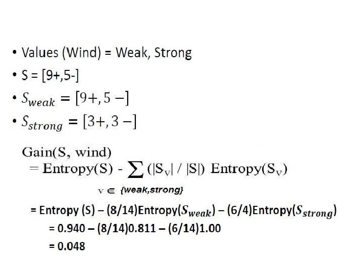
INFORMATION GAIN MEASURES THE EXPECTED REDUCTION IN ENTROPY Information gain is the expected reduction in entropy caused by partitioning the examples according to some attribute A Split the node with attribute having highest Gain • S – a collection of examples • A – an attribute • Values(A) – possible values of attribute A; • Sv– the subset of S for which attribute A has value v.

ID 3 using Information Gain

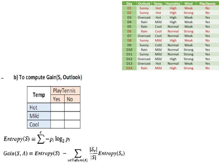
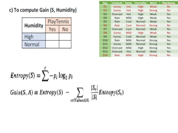
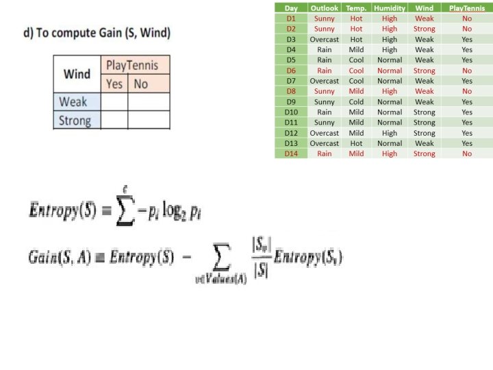
ID 3: Illustration Day Outlook Temp. Humidity Wind Play. Tennis D 1 Sunny Hot High Weak No D 2 Sunny Hot High Strong No D 3 Overcast Hot High Weak Yes D 4 Rain Mild High Weak Yes D 5 Rain Cool Normal Weak Yes D 6 Rain Cool Normal Strong No D 7 Overcast Cool Normal Weak Yes D 8 Sunny Mild High Weak No D 9 Sunny Cold Normal Weak Yes D 10 Rain Mild Normal Strong Yes D 11 Sunny Mild Normal Strong Yes D 12 Overcast Mild High Strong Yes D 13 Overcast Hot Normal Weak Yes D 14 Rain Mild High Strong No

1. Level 0: To identify Root Node Entropy(S) =

Illustration

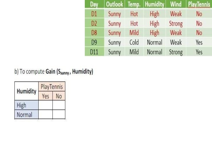
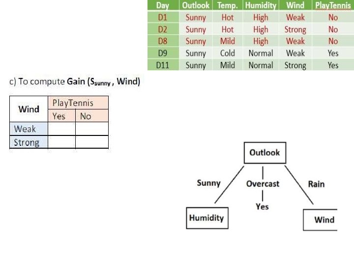
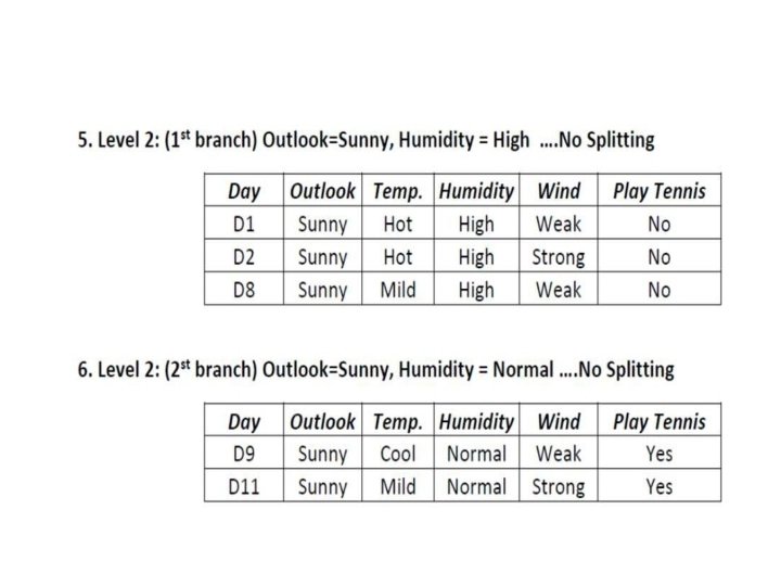
2. Level 1: (1 st branch) Outlook=Sunny • Entropy(Ssunny) =

3. Level 1: (2 nd branch) Outlook = Overcast, All are yes, No Splitting required.

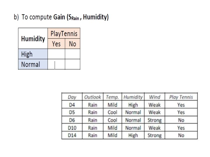
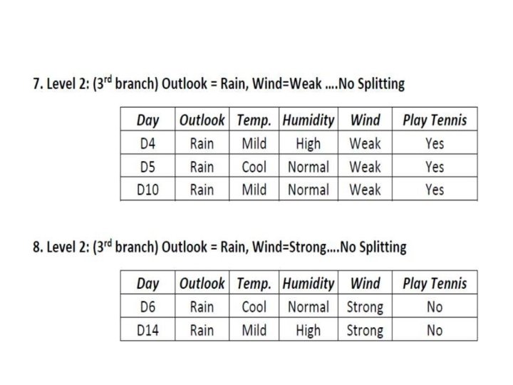
Illustration 4. Level 1: (3 rd branch) Outlook = Rain • Entropy(Srain)

Illustration: Final Decision Tree

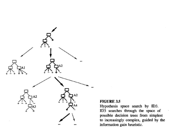
HYPOTHESIS SPACE SEARCH IN DECISION TREE LEARNING • The hypothesis space searched by ID 3 is the set of possible decision trees. • ID 3 performs a simple-to complex, hill-climbing search through this hypothesis space, beginning with the empty tree, then considering progressively more elaborate hypotheses in search of a decision tree that correctly classifies the training data. • The evaluation function that guides this hill-climbing search is the information gain measure.

Capabilities and Limitations of ID 3 • ID 3’s hypothesis space of all decision trees is a complete space of finite discrete-valued functions, relative to the available attributes. • ID 3 maintains only a single current hypothesis as it searches through the space of decision trees. • ID 3 in its pure form performs no backtracking in its search. Once it selects an attribute to test at a particular level in the tree, it never backtracks to reconsider this choice. • ID 3 uses all training examples at each step in the search to make statistically based decisions regarding how to refine its current hypothesis. This contrasts with methods that make decisions incrementally, based on individual training examples (e. g. , FIND-So r CANDIDATE-ELIMINA

INDUCTIVE BIAS IN DECISION TREE LEARNING • Inductive bias is the set of assumptions that, together with the training data, deductively justify the classifications assigned by the learner to future instances. • Typically there are many decision trees consistent with training examples. • It chooses the first acceptable tree it encounters in its simple- to-complex, hill-climbing search through the space of possible trees • Approximate inductive bias of ID 3: Shorter trees are preferred over larger trees. • A closer approximation to the inductive bias of ID 3 –Shorter trees are preferred over longer trees. –Trees that place high information gain attributes close to the root are preferred over those that do not

Restriction Biases and Preference Biases The inductive bias of ID 3 is thus a preference for certain hypotheses over others (e. g. , for shorter hypotheses) • This form of bias is typically called a preference bias (or, alternatively, a search bias). In contrast, the bias of the CEA is in the form of a categorical restriction on the set of hypotheses considered. • This form of bias is typically called a restriction bias (or, alternatively, a language bias). A preference bias is more desirable than a restriction bias ID 3 exhibits a purely preference bias and CEA is a purely restriction bias whereas some learning systems combine both.

Why prefer short hypothesis? Occam's razor: (Problem Solving Principle) • Prefer the simplest hypothesis that fits the data. • (The term razor is frequency and effectiveness with which he used it)

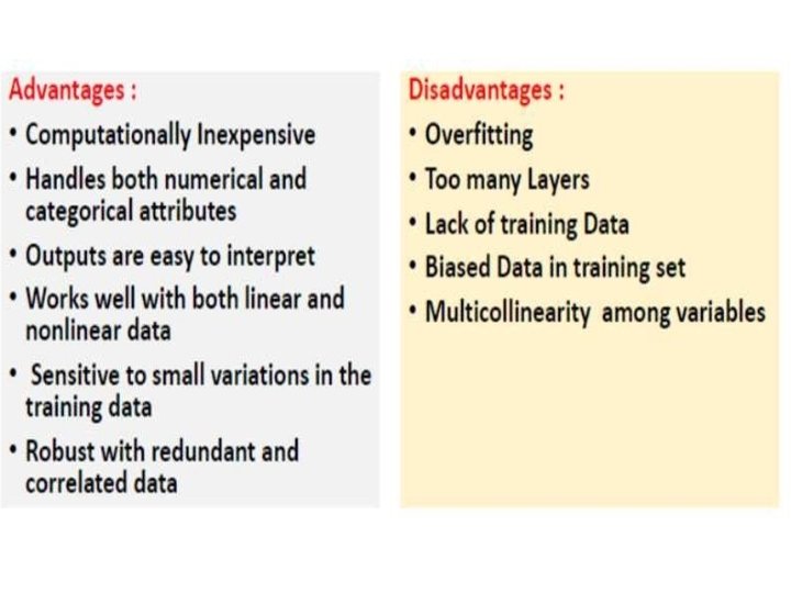
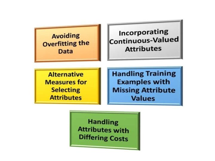
Issues in Decision tree learning Practical issues in learning decision trees include • determining how deeply to grow the decision tree, • handling continuous attributes, • choosing an appropriate attribute selection measure, • handling training data with missing attribute values, • handling attributes with differing costs, and • improving computational efficiency. we discuss each of these issues and extensions to the basic ID 3 algorithm that address them. ID 3 has itself been extended to address most of these issues, with the resulting system renamed C 4. 5.

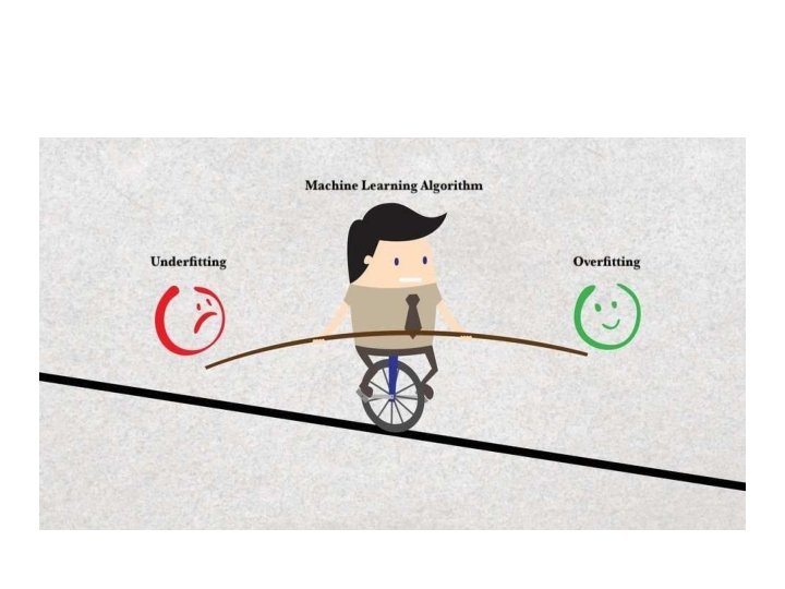
Overfitting Consider 2 D data. +ve examples are plotted in Blue, -ve are in Red The green line represents an overfitted model and the black line represents a regularized model. While the green line best follows the training data, it is too dependent on that data and it is likely to have a higher error rate on new unseen data, compared to the black line.

• Definition: Given a hypothesis space H, a hypothesis h E H is said to overfit the training data if there exists some alternative hypothesis h' E H, such that h has smaller error than h' over the training examples, but h' has a smaller error than h over the entire distribution of instances • Underfitting: Underfitting occurs when a statistical model cannot adequately capture the underlying structure of the data.

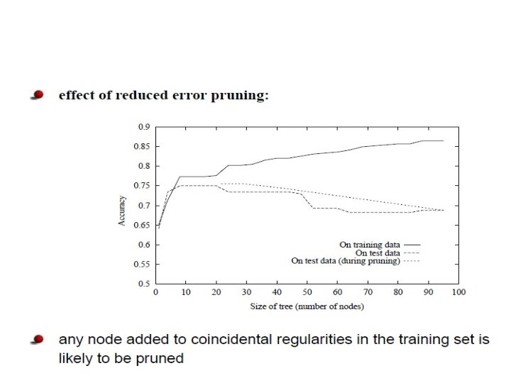
• Validation Set How exactly might we use a validation set to prevent overfitting? • Reduced Error Pruning • Rule Post-Pruning is a technique in machine learning that reduces the size of decision trees by removing sections of the tree that provide little power to classify instances. Pruning reduces the complexity of the final classifier, and hence improves predictive accuracy by the reduction of overfitting.

Reduced Error Pruning

RULE POST-PRUNING • In practice, one quite successful method for finding high accuracy hypotheses is a technique we shall call rule post-pruning. A variant of this pruning method is used by C 4. 5 (Quinlan 1993), which is an outgrowth of the original ID 3 algorithm. • Rule post-pruning involves the following steps: 1. Infer the decision tree from the training set, growing the tree until the training data is fit as well as possible and allowing overfitting to occur. 2. Convert the learned tree into an equivalent set of rules by creating one rule for each path from the root node to a leaf node. 3. Prune (generalize) each rule by removing any preconditions that result in improving its estimated accuracy. 4. Sort the pruned rules by their estimated accuracy, and consider them in this sequence when classifying subsequent instances.

• To illustrate, consider again the decision tree. In rule postpruning, one rule is generated for each leaf node in the tree. • Each attribute test along the path from the root to the leaf becomes a rule antecedent (precondition) • and the classification at the leaf node becomes the rule consequent (postcondition). • For example, the leftmost path of the tree in Figure 3. 1 is translated into the rule IF (Outlook = Sunny) A (Humidity = High) THEN Play. Tennis = No

Why convert the decision tree to rules before pruning? There are three main advantages. • Converting to rules allows distinguishing among the different contexts in which a decision node is used. Because each distinct path through the decision tree node produces a distinct rule, the pruning decision regarding that attribute test can be made differently for each path. In contrast, if the tree itself were pruned, the only two choices would be to remove the decision node completely, or to retain its original form. • Converting to rules removes the distinction between attribute tests that occur near the root of the tree and those that occur near the leaves. Thus, we avoid messy bookkeeping issues such as how to reorganize the tree if the root node is pruned while retaining part of the subtree below this test. • Converting to rules improves readability. Rules are often

Issue No. : 2 Incorporating Continuous-Valued Attributes

example

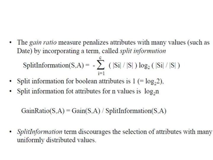
Alternative Measures for Selecting Attributes

Practical issues on Split information

Issue 4: Handling Training Examples with Missing Attribute Values

Issue 5: Handling Attributes with Differing Costs