Data Analysis Overview Experimental environment System Config parameters

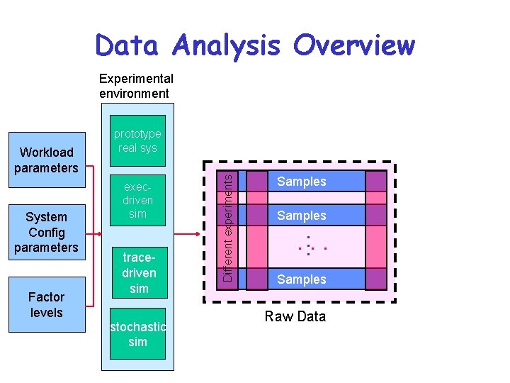
Data Analysis Overview Experimental environment System Config parameters Factor levels execdriven sim tracedriven sim stochastic sim Different experiments Workload parameters prototype real sys Samples . . . Samples Raw Data

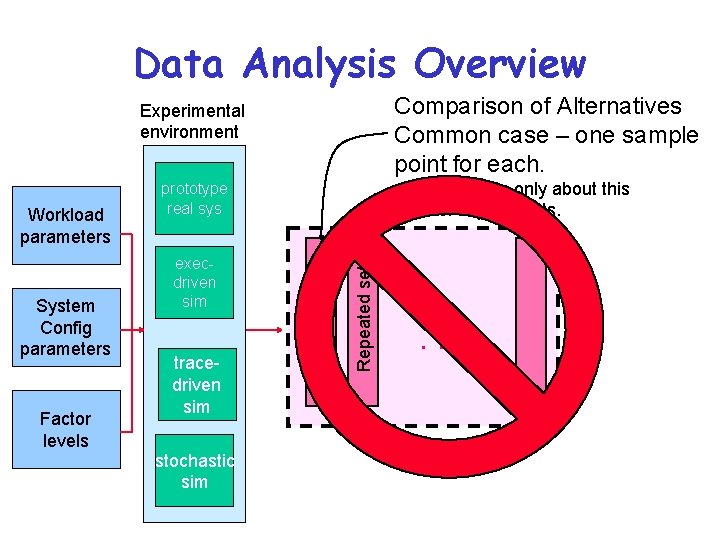
Data Analysis Overview Comparison of Alternatives Common case – one sample point for each. Experimental environment Factor levels tracedriven sim stochastic sim Repeated set System Config parameters execdriven sim 1 set of experiments Workload parameters • Conclusions only about this set of experiments. prototype real sys . . . Raw Data

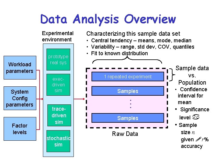
Data Analysis Overview Experimental environment Workload parameters System Config parameters Factor levels prototype real sys execdriven sim tracedriven sim stochastic sim Characterizing this sample data set • Central tendency – means, mode, median • Variability – range, std dev, COV, quantiles • Fit to known distribution 1 repeated experiment Samples . . . Samples Raw Data Sample data vs. Population • Confidence interval for mean • Significance level a • Sample size n given !r% accuracy

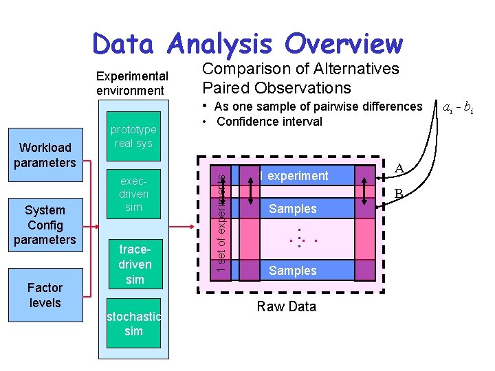
Data Analysis Overview Experimental environment Comparison of Alternatives Paired Observations • As one sample of pairwise differences System Config parameters Factor levels execdriven sim tracedriven sim stochastic sim • Confidence interval 1 set of experiments Workload parameters prototype real sys 1 experiment A B Samples . . . Samples Raw Data ai - bi

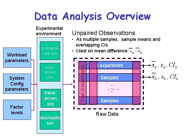
Data Analysis Overview Workload parameters System Config parameters Factor levels prototype real sys execdriven sim tracedriven sim stochastic sim Unpaired Observations • As multiple samples, sample means and overlapping CIs • t-test on mean difference: xa - xb 1 set of experiments Experimental environment 1 experiment xa , sa , CIa Samples xb , sb , CIb . . . Samples Raw Data

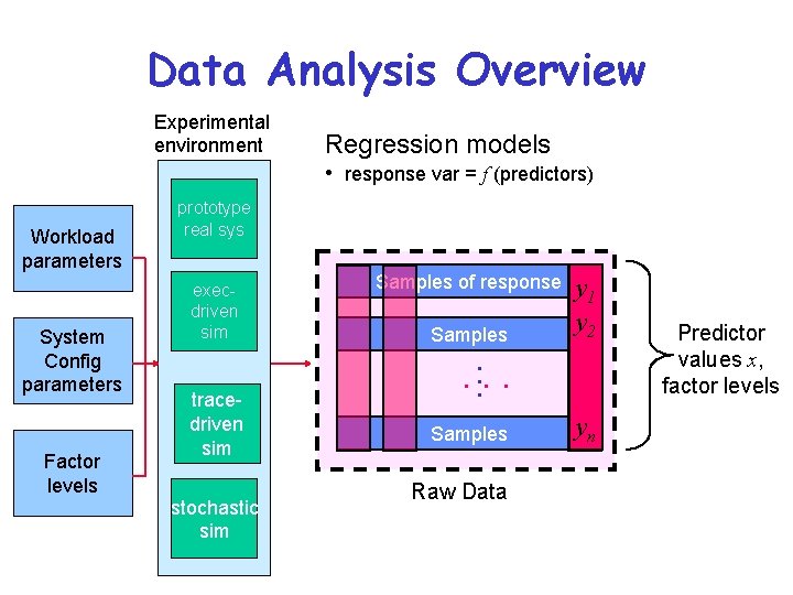
Data Analysis Overview Experimental environment Regression models • response var = f (predictors) Workload parameters System Config parameters Factor levels prototype real sys execdriven sim Samples of response Samples y 1 y 2 . tracedriven sim stochastic sim . . . Samples Raw Data yn Predictor values x, factor levels

Linear Regression Models ü What is a (good) model? ü Estimating model parameters ü Allocating variation (R 2) • Confidence intervals for regressions ü Verifying assumptions visually © 1998, Geoff Kuenning

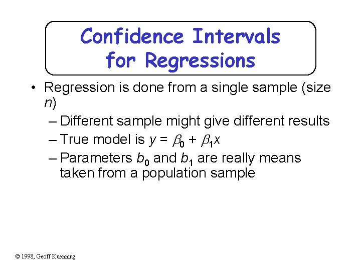
Confidence Intervals for Regressions • Regression is done from a single sample (size n) – Different sample might give different results – True model is y = 0 + 1 x – Parameters b 0 and b 1 are really means taken from a population sample © 1998, Geoff Kuenning

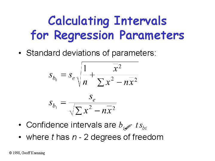
Calculating Intervals for Regression Parameters • Standard deviations of parameters: • Confidence intervals are bi t sbi • where t has n - 2 degrees of freedom ! © 1998, Geoff Kuenning

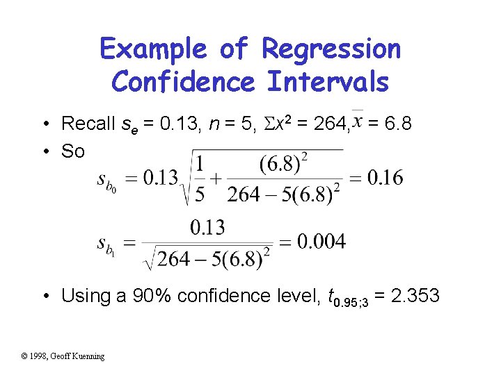
Example of Regression Confidence Intervals • Recall se = 0. 13, n = 5, x 2 = 264, = 6. 8 • So • Using a 90% confidence level, t 0. 95; 3 = 2. 353 © 1998, Geoff Kuenning

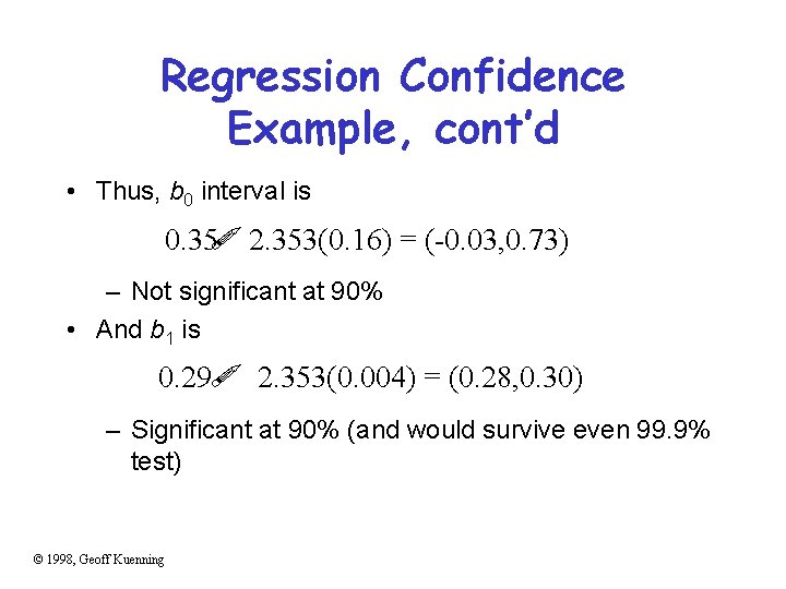
Regression Confidence Example, cont’d • Thus, b 0 interval is ! 0. 35 2. 353(0. 16) = (-0. 03, 0. 73) – Not significant at 90% • And b 1 is ! 0. 29 2. 353(0. 004) = (0. 28, 0. 30) – Significant at 90% (and would survive even 99. 9% test) © 1998, Geoff Kuenning

Confidence Intervals for Predictions • Previous confidence intervals are for parameters – How certain can we be that the parameters are correct? • Purpose of regression is prediction – How accurate are the predictions? – Regression gives mean of predicted response, based on sample we took © 1998, Geoff Kuenning

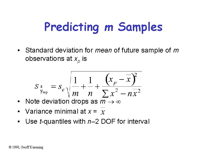
Predicting m Samples • Standard deviation for mean of future sample of m observations at xp is S N ymp • Note deviation drops as m • Variance minimal at x = • Use t-quantiles with n– 2 DOF for interval © 1998, Geoff Kuenning

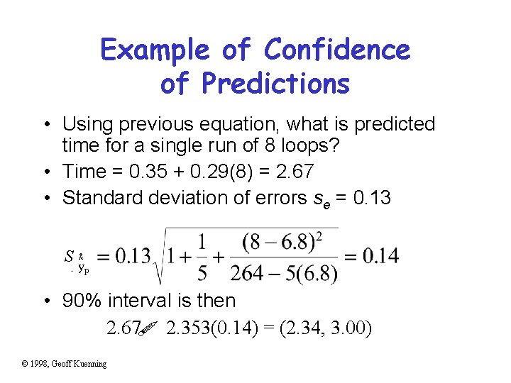
Example of Confidence of Predictions • Using previous equation, what is predicted time for a single run of 8 loops? • Time = 0. 35 + 0. 29(8) = 2. 67 • Standard deviation of errors se = 0. 13 S N yp • 90% interval is then 2. 67 2. 353(0. 14) = (2. 34, 3. 00) ! © 1998, Geoff Kuenning

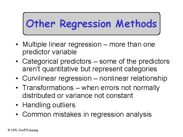
Other Regression Methods • Multiple linear regression – more than one predictor variable • Categorical predictors – some of the predictors aren’t quantitative but represent categories • Curvilinear regression – nonlinear relationship • Transformations – when errors not normally distributed or variance not constant • Handling outliers • Common mistakes in regression analysis © 1998, Geoff Kuenning

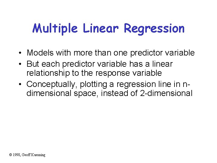
Multiple Linear Regression • Models with more than one predictor variable • But each predictor variable has a linear relationship to the response variable • Conceptually, plotting a regression line in ndimensional space, instead of 2 -dimensional © 1998, Geoff Kuenning

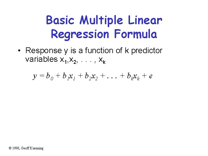
Basic Multiple Linear Regression Formula • Response y is a function of k predictor variables x 1, x 2, . . . , xk y = b 0 + b 1 x 1 + b 2 x 2 +. . . + bkxk + e © 1998, Geoff Kuenning

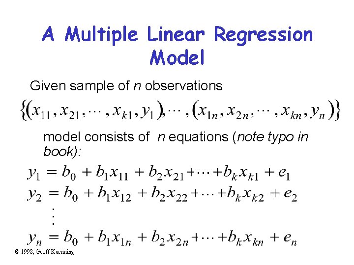
A Multiple Linear Regression Model Given sample of n observations. . model consists of n equations (note typo in book): . . . © 1998, Geoff Kuenning

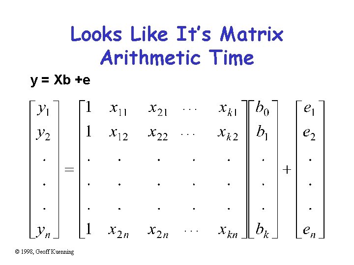
Looks Like It’s Matrix Arithmetic Time y = Xb +e. . © 1998, Geoff Kuenning

Analysis of Multiple Linear Regression • Listed in box 15. 1 of Jain • Not terribly important (for our purposes) how they were derived – This isn’t a class on statistics • But you need to know how to use them • Mostly matrix analogs to simple linear regression results © 1998, Geoff Kuenning

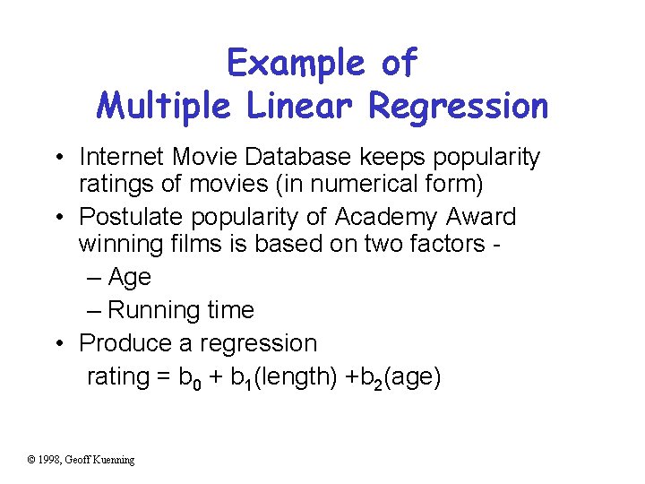
Example of Multiple Linear Regression • Internet Movie Database keeps popularity ratings of movies (in numerical form) • Postulate popularity of Academy Award winning films is based on two factors – Age – Running time • Produce a regression rating = b 0 + b 1(length) +b 2(age) © 1998, Geoff Kuenning

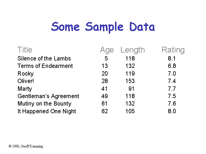
Some Sample Data Title Age Length Silence of the Lambs Terms of Endearment Rocky Oliver! Marty Gentleman’s Agreement Mutiny on the Bounty It Happened One Night 5 13 20 28 41 49 61 62 © 1998, Geoff Kuenning 118 132 119 153 91 118 132 105 Rating 8. 1 6. 8 7. 0 7. 4 7. 7 7. 5 7. 6 8. 0

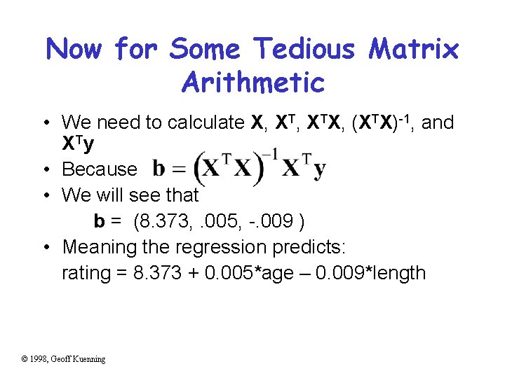
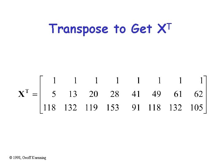
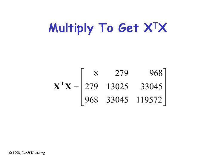
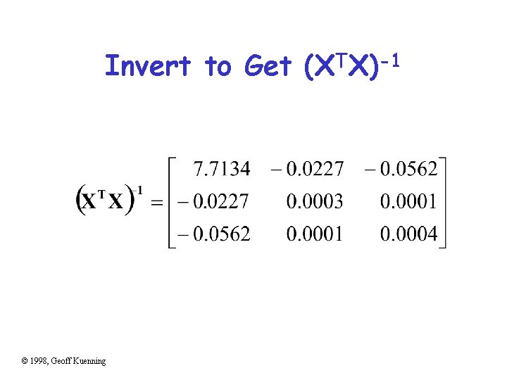
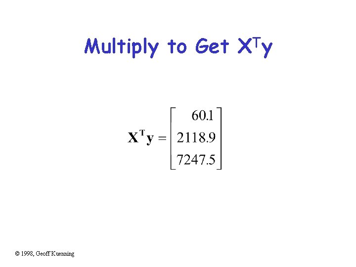
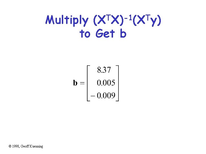
Now for Some Tedious Matrix Arithmetic • We need to calculate X, XTX, (XTX)-1, and X Ty • Because • We will see that b = (8. 373, . 005, -. 009 ) • Meaning the regression predicts: rating = 8. 373 + 0. 005*age – 0. 009*length © 1998, Geoff Kuenning

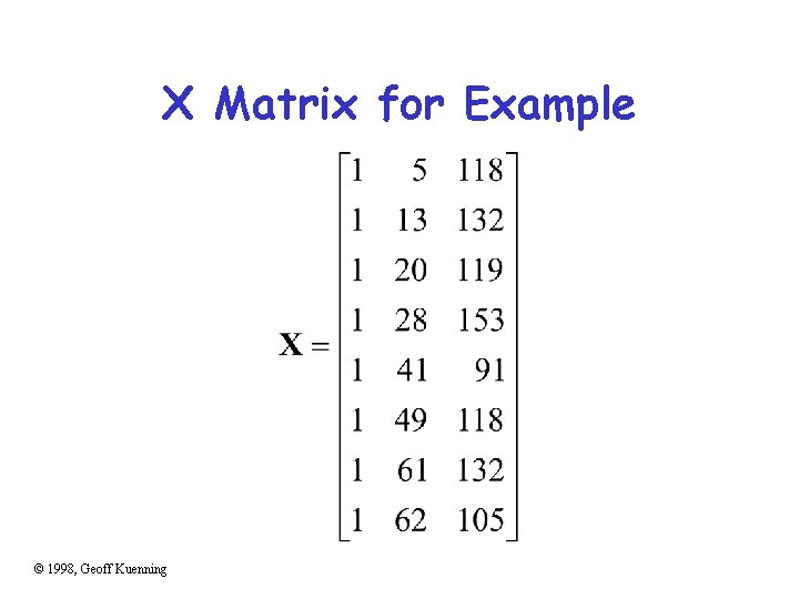
X Matrix for Example © 1998, Geoff Kuenning

Transpose to Get XT © 1998, Geoff Kuenning

Multiply To Get XTX © 1998, Geoff Kuenning

Invert to Get (XTX)-1 © 1998, Geoff Kuenning

Multiply to Get XTy © 1998, Geoff Kuenning

Multiply (XTX)-1(XTy) to Get b © 1998, Geoff Kuenning

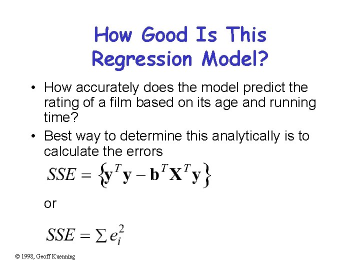
How Good Is This Regression Model? • How accurately does the model predict the rating of a film based on its age and running time? • Best way to determine this analytically is to calculate the errors or © 1998, Geoff Kuenning

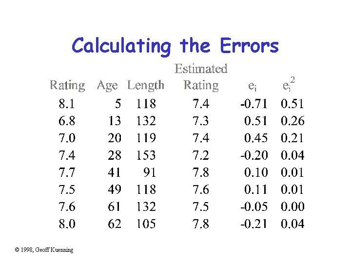
Calculating the Errors © 1998, Geoff Kuenning

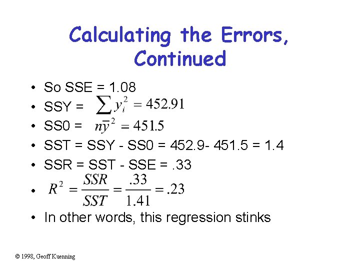
Calculating the Errors, Continued • • • So SSE = 1. 08 SSY = SS 0 = SST = SSY - SS 0 = 452. 9 - 451. 5 = 1. 4 SSR = SST - SSE =. 33 • • In other words, this regression stinks © 1998, Geoff Kuenning

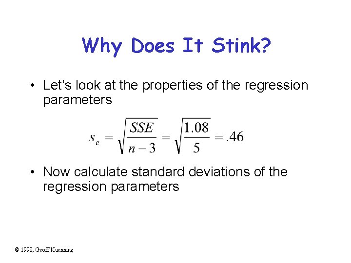
Why Does It Stink? • Let’s look at the properties of the regression parameters • Now calculate standard deviations of the regression parameters © 1998, Geoff Kuenning

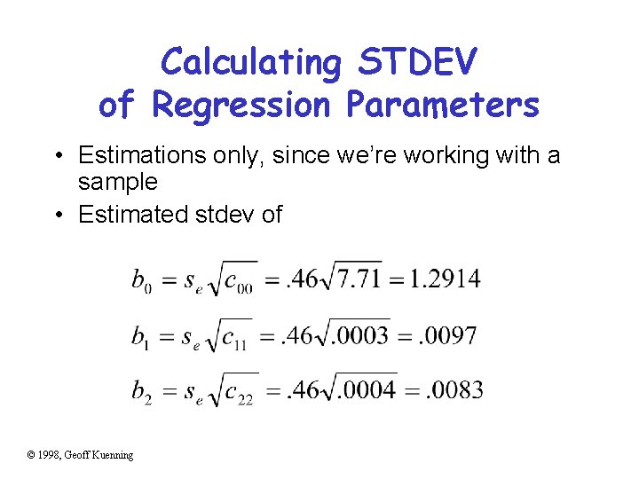
Calculating STDEV of Regression Parameters • Estimations only, since we’re working with a sample • Estimated stdev of © 1998, Geoff Kuenning

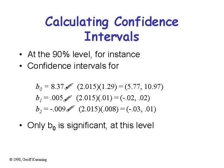
Calculating Confidence Intervals • At the 90% level, for instance • Confidence intervals for ! ! ! b 0 = 8. 37 b 1 =. 005 b 2 = -. 009 (2. 015)(1. 29) = (5. 77, 10. 97) (2. 015)(. 01) = (-. 02, . 02) (2. 015)(. 008) = (-. 03, . 01) • Only b 0 is significant, at this level © 1998, Geoff Kuenning

Analysis of Variance • So, can we really say that none of the predictor variables are significant? – Not yet; predictors may be correlated • F-test can be used for this purpose – E. g. , to determine if the SSR is significantly higher than the SSE – Equivalent to testing that y does not depend on any of the predictor variables © 1998, Geoff Kuenning

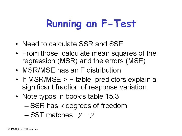
Running an F-Test • Need to calculate SSR and SSE • From those, calculate mean squares of the regression (MSR) and the errors (MSE) • MSR/MSE has an F distribution • If MSR/MSE > F-table, predictors explain a significant fraction of response variation • Note typos in book’s table 15. 3 – SSR has k degrees of freedom – SST matches © 1998, Geoff Kuenning

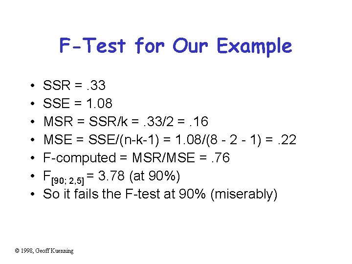
F-Test for Our Example • • SSR =. 33 SSE = 1. 08 MSR = SSR/k =. 33/2 =. 16 MSE = SSE/(n-k-1) = 1. 08/(8 - 2 - 1) =. 22 F-computed = MSR/MSE =. 76 F[90; 2, 5] = 3. 78 (at 90%) So it fails the F-test at 90% (miserably) © 1998, Geoff Kuenning

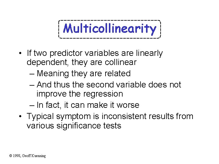
Multicollinearity • If two predictor variables are linearly dependent, they are collinear – Meaning they are related – And thus the second variable does not improve the regression – In fact, it can make it worse • Typical symptom is inconsistent results from various significance tests © 1998, Geoff Kuenning

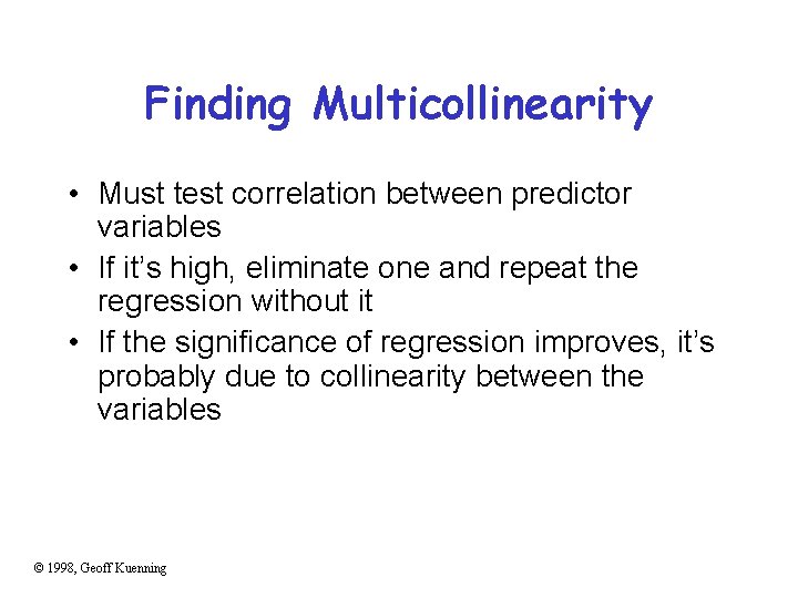
Finding Multicollinearity • Must test correlation between predictor variables • If it’s high, eliminate one and repeat the regression without it • If the significance of regression improves, it’s probably due to collinearity between the variables © 1998, Geoff Kuenning

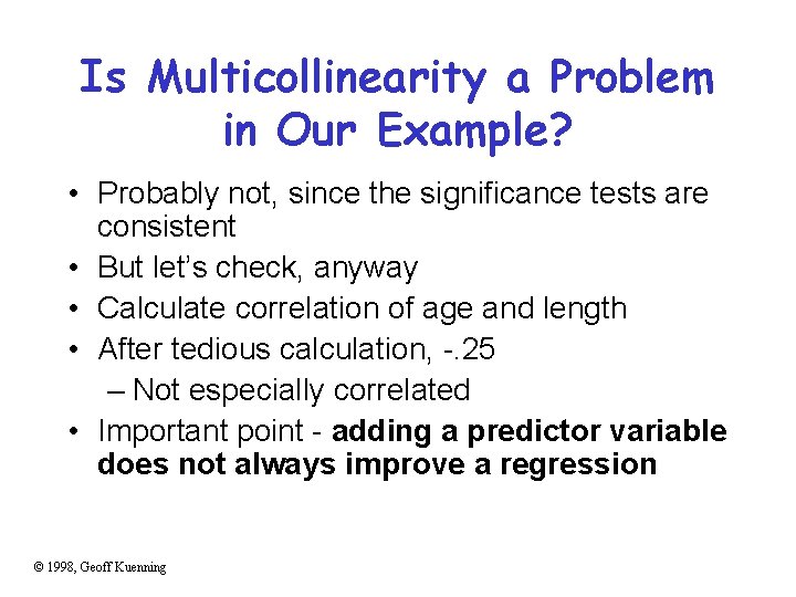
Is Multicollinearity a Problem in Our Example? • Probably not, since the significance tests are consistent • But let’s check, anyway • Calculate correlation of age and length • After tedious calculation, -. 25 – Not especially correlated • Important point - adding a predictor variable does not always improve a regression © 1998, Geoff Kuenning

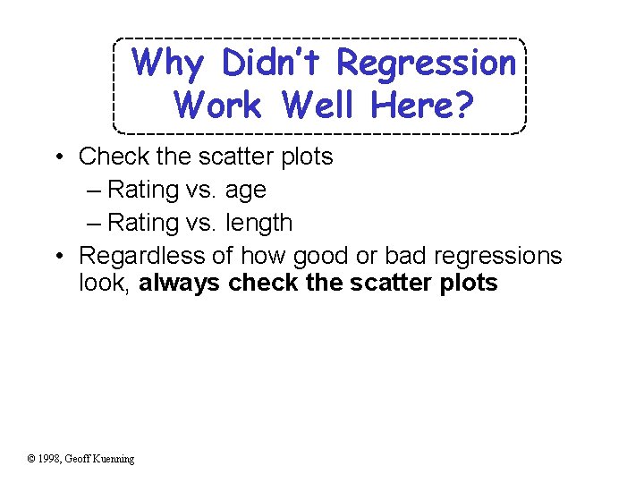
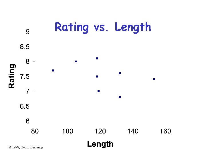
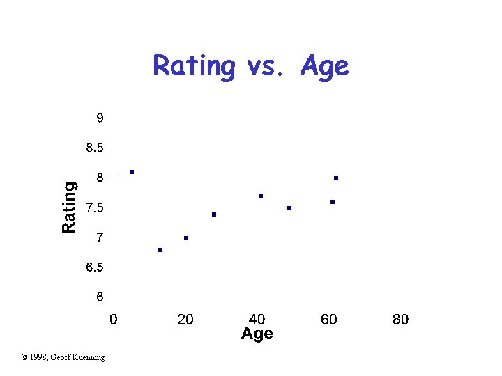
Why Didn’t Regression Work Well Here? • Check the scatter plots – Rating vs. age – Rating vs. length • Regardless of how good or bad regressions look, always check the scatter plots © 1998, Geoff Kuenning

Rating vs. Length © 1998, Geoff Kuenning

Rating vs. Age © 1998, Geoff Kuenning

Regression With Categorical Predictors • Regression methods discussed so far assume numerical variables • What if some of your variables are categorical in nature? • Use techniques discussed later in the class if all predictors are categorical • Levels - number of values a category can take © 1998, Geoff Kuenning

Handling Categorical Predictors • If only two levels, define bi as follows – bi = 0 for first value – bi = 1 for second value • This definition is missing from book in section 15. 2 • Can use +1 and -1 as values, instead • Need k-1 predictor variables for k levels – To avoid implying order in categories © 1998, Geoff Kuenning

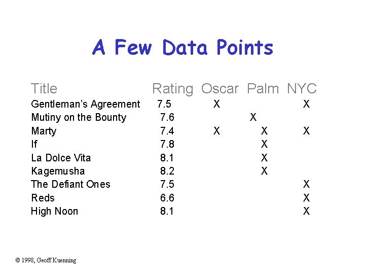
Categorical Variables Example • Which is a better predictor of a high rating in the movie database, winning an Oscar, winning the Golden Palm at Cannes, or winning the New York Critics Circle? © 1998, Geoff Kuenning

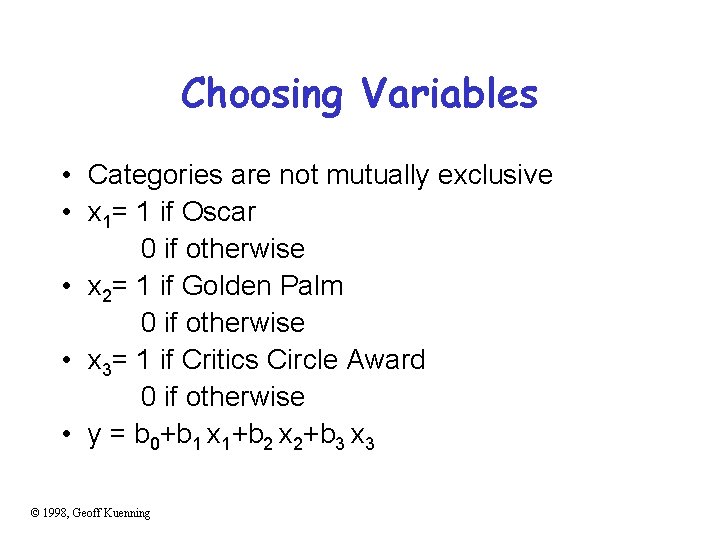
Choosing Variables • Categories are not mutually exclusive • x 1= 1 if Oscar 0 if otherwise • x 2= 1 if Golden Palm 0 if otherwise • x 3= 1 if Critics Circle Award 0 if otherwise • y = b 0+b 1 x 1+b 2 x 2+b 3 x 3 © 1998, Geoff Kuenning

A Few Data Points Title Gentleman’s Agreement Mutiny on the Bounty Marty If La Dolce Vita Kagemusha The Defiant Ones Reds High Noon © 1998, Geoff Kuenning Rating Oscar Palm NYC 7. 5 7. 6 7. 4 7. 8 8. 1 8. 2 7. 5 6. 6 8. 1 X X X

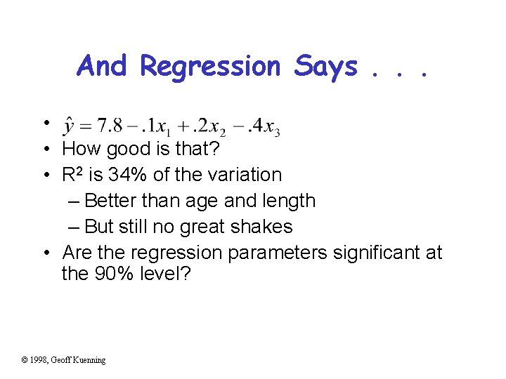
And Regression Says. . . • • How good is that? • R 2 is 34% of the variation – Better than age and length – But still no great shakes • Are the regression parameters significant at the 90% level? © 1998, Geoff Kuenning

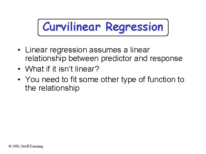
Curvilinear Regression • Linear regression assumes a linear relationship between predictor and response • What if it isn’t linear? • You need to fit some other type of function to the relationship © 1998, Geoff Kuenning

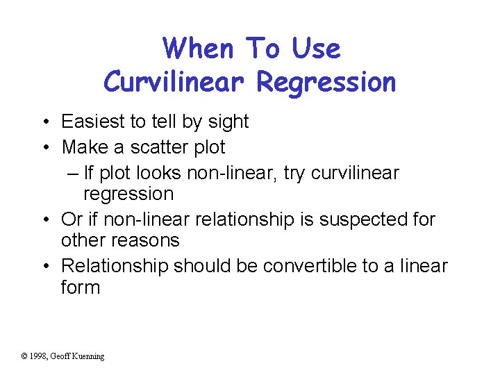
When To Use Curvilinear Regression • Easiest to tell by sight • Make a scatter plot – If plot looks non-linear, try curvilinear regression • Or if non-linear relationship is suspected for other reasons • Relationship should be convertible to a linear form © 1998, Geoff Kuenning

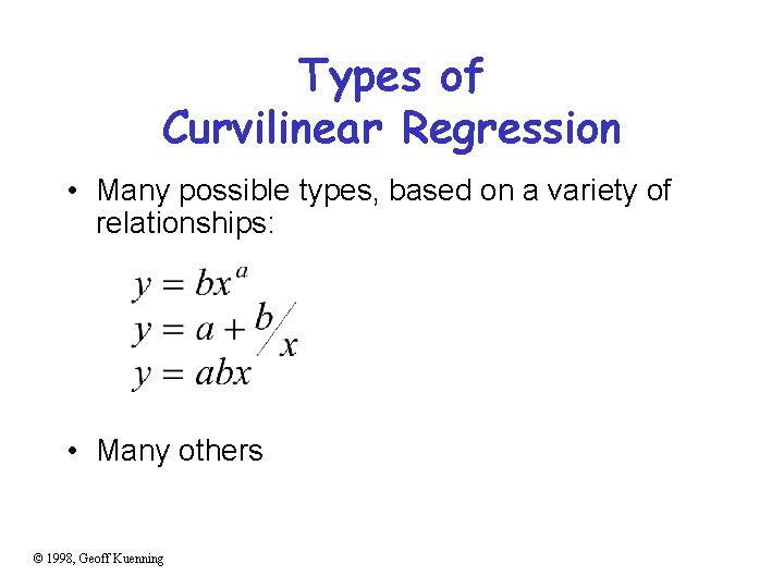
Types of Curvilinear Regression • Many possible types, based on a variety of relationships: • Many others © 1998, Geoff Kuenning

Transform Them to Linear Forms • Apply logarithms, multiplication, division, whatever to produce something in linear form • I. e. , y = a + b*something • Or a similar form • If predictor appears in more than one transformed predictor variable, correlation likely © 1998, Geoff Kuenning

Transformations • Using some function of the response variable y in place of y itself • Curvilinear regression is one example of transformation • But techniques are more generally applicable © 1998, Geoff Kuenning

When To Transform? • If known properties of the measured system suggest it • If the data’s range covers several orders of magnitude • If the homogeneous variance assumption of the residuals is violated © 1998, Geoff Kuenning

Transforming Due To Homoscedasticity • If spread of scatter plot of residual vs. predicted response is not homogeneous, • Then residuals are still functions of the predictor variables • Transformation of response may solve the problem © 1998, Geoff Kuenning

What Transformation To Use? • Compute standard deviation of the residuals • Plot as function of the mean of the observations – Assuming multiple experiments for single set of predictor values • Check for linearity - if it is, use a log transform © 1998, Geoff Kuenning

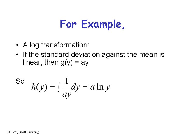
Other Tests for Transformations • If variance against mean of observations is linear, use square root transform • If standard deviation against mean squared is linear, use inverse transform • If standard deviation against mean to a power is linear, use a power transform • More covered in the book © 1998, Geoff Kuenning

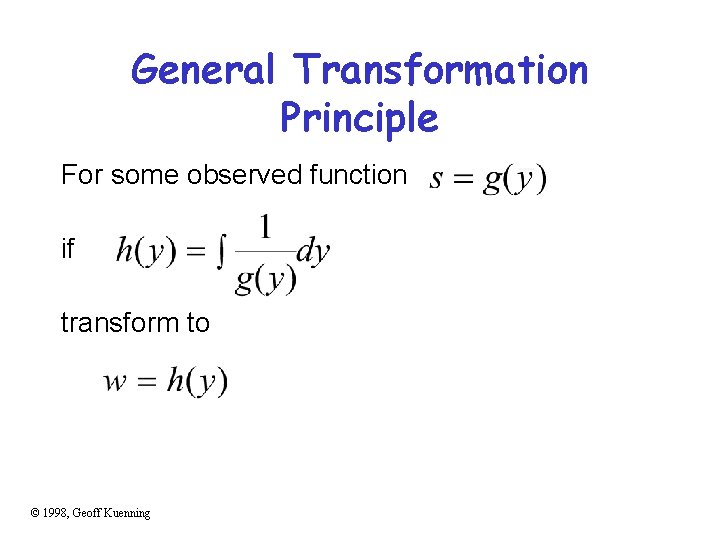
General Transformation Principle For some observed function if transform to © 1998, Geoff Kuenning

For Example, • A log transformation: • If the standard deviation against the mean is linear, then g(y) = ay So © 1998, Geoff Kuenning

Outliers • Atypical observations might be outliers – Measurements that are not truly characteristic – By chance, several standard deviations out – Or mistakes might have been made in measurement • Which leads to a problem: Do you include outliers in analysis or not? © 1998, Geoff Kuenning

Deciding How To Handle Outliers 1. Find them (by looking at scatter plot) 2. Check carefully for experimental error 3. Repeat experiments at predictor values for the outlier 4. Decide whether to include or not include outliers – Or do analysis both ways Question: Is the first point in the example an outlier on the rating vs. age plot? © 1998, Geoff Kuenning

Common Mistakes in Regression • Generally based on taking shortcuts • Or not being careful • Or not understanding some fundamental principles of statistics © 1998, Geoff Kuenning

Not Verifying Linearity • Draw the scatter plot • If it isn’t linear, check for curvilinear possibilities • Using linear regression when the relationship isn’t linear is misleading © 1998, Geoff Kuenning

Relying on Results Without Visual Verification • Always check the scatter plot as part of regression – Examining the line regression predicts vs. the actual points • Particularly important if regression is done automatically © 1998, Geoff Kuenning

Attaching Importance To Values of Parameters • Numerical values of regression parameters depend on scale of predictor variables • So just because a particular parameter’s value seems “small” or “large, ” not necessarily an indication of importance • E. g. , converting seconds to microseconds doesn’t change anything fundamental – But magnitude of associated parameter changes © 1998, Geoff Kuenning

Not Specifying Confidence Intervals • Samples of observations are random • Thus, regression performed on them yields parameters with random properties • Without a confidence interval, it’s impossible to understand what a parameter really means © 1998, Geoff Kuenning

Not Calculating Coefficient of Determination • Without R 2, difficult to determine how much of variance is explained by the regression • Even if R 2 looks good, safest to also perform an F-test • The extra amount of effort isn’t that large, anyway © 1998, Geoff Kuenning

Using Coefficient of Correlation Improperly • Coefficient of determination is R 2 • Coefficient of correlation is R • R 2 gives percentage of variance explained by regression, not R • E. g. , if R is. 5, R 2 is. 25 – And the regression explains 25% of variance – Not 50% © 1998, Geoff Kuenning

Using Highly Correlated Predictor Variables • If two predictor variables are highly correlated, using both degrades regression • E. g. , likely to be a correlation between an executable’s on-disk size and in-core size – So don’t use both as predictors of run time • Which means you need to understand your predictor variables as well as possible © 1998, Geoff Kuenning

Using Regression Beyond Range of Observations • Regression is based on observed behavior in a particular sample • Most likely to predict accurately within range of that sample – Far outside the range, who knows? • E. g. , a regression on run time of executables that are smaller than size of main memory may not predict performance of executables that require much VM activity © 1998, Geoff Kuenning

Using Too Many Predictor Variables • Adding more predictors does not necessarily improve the model • More likely to run into multicollinearity problems • So what variables to choose? – Subject of much of this course © 1998, Geoff Kuenning

Measuring Too Little of the Range • Regression only predicts well near range of observations • If you don’t measure the commonly used range, regression won’t predict much • E. g. , if many programs are bigger than main memory, only measuring those that are smaller is a mistake © 1998, Geoff Kuenning

Assuming Good Predictor Is a Good Controller • Correlation isn’t necessarily control • Just because variable A is related to variable B, you may not be able to control values of B by varying A • E. g. , if number of hits on a Web page and server bandwidth are correlated, you might not increase hits by increasing bandwidth • Often, a goal of regression is finding control variables © 1998, Geoff Kuenning

For Discussion Today Project Proposal 1. Statement of hypothesis 2. Workload decisions 3. Metrics to be used 4. Method