CS 6501 3 D Reconstruction and Understanding Feature


 Slide from Fei Li, Juan Carlos Niebles")
 Slide from Fei Li, Juan Carlos Niebles, Steve Seitz")


 in a window")


 • 3 D photography /")

![Gaussian Pyramids Known as a Gaussian Pyramid [Burt and Adelson, 1983] • In computer](https://slidetodoc.com/presentation_image_h2/eefa8e3e45011885b28fec6b5c07309b/image-25.jpg "Gaussian Pyramids Known as a Gaussian Pyramid [Burt and Adelson, 1983] • In computer")


 suppression • Detect maxima and minima of difference-of. Gaussian in scale space")


 • Next question:")


 • Image gradients are sampled over 16 x 16")
 • Often “SIFT” = • Difference of Gaussian keypoint")


![Feature-space outlier rejection • From [Lowe, 1999]: • 1 -NN: SSD of the closest](https://slidetodoc.com/presentation_image_h2/eefa8e3e45011885b28fec6b5c07309b/image-41.jpg "Feature-space outlier rejection • From [Lowe, 1999]: • 1 -NN: SSD of the closest")


 Slide from Silvio Savarese")


![Hough Transform: Effect of Noise [Forsyth & Ponce]](https://slidetodoc.com/presentation_image_h2/eefa8e3e45011885b28fec6b5c07309b/image-55.jpg "Hough Transform: Effect of Noise [Forsyth & Ponce]")


 : Fischler & Bolles in ‘ 81. Algorithm: 1. Sample")
 the number of points required to")
 the number of points required to")
 the number of points required to")
 the number of points required to fit the model")


 • Fit a model placing")


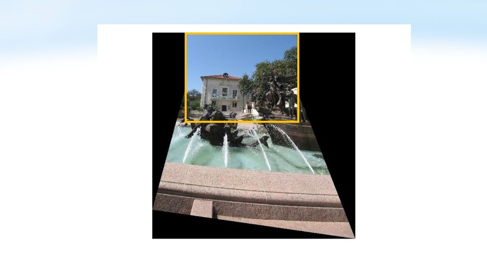


 2. Warp the other images towards it")

- Slides: 84
CS 6501: 3 D Reconstruction and Understanding Feature Detection and Matching Connelly Barnes Slides from Jason Lawrence, Fei Li, Juan Carlos Niebles, Alexei Efros, Rick Szeliski, Fredo Durand, Kristin Grauman, James Hays
Outline • • • Motivation for sparse features Harris corner detector Difference of Gaussian (blob) feature detector Sparse feature descriptor: SIFT Robust model fitting • Hough transform • RANSAC • Application: panorama stitching
Motivation: Image Matching (Hard Problem) Slide from Fei Li, Juan Carlos Niebles
Motivation: Image Matching (Harder Case) Slide from Fei Li, Juan Carlos Niebles, Steve Seitz
What is a Feature? • In computer vision, a feature refers to a region of interest in an image: typically, low-level features, such as corner, edge, blob. Corner features Slide from Krystian Mikolajczyk
Motivation for sparse/local features • Global features can only summarize the overall content of the image. • Local (or sparse) features can allow us to match local regions with more geometric accuracy. • Increased robustness to: Slide from Fei Li, Juan Carlos Niebles
Motivating Application: Panorama Stitching • Are you getting the whole picture? • Compact Camera FOV = 50 x 35° Slide from Brown & Lowe
Motivating Application: Panorama Stitching • Are you getting the whole picture? • Compact Camera FOV = 50 x 35° • Human FOV = 200 x 135° Slide from Brown & Lowe
Motivating Application: Panorama Stitching • Are you getting the whole picture? • Compact Camera FOV = 50 x 35° • Human FOV = 200 x 135° • Panoramic Mosaic = 360 x 180° Slide from Brown & Lowe
Mosaics: stitching images together virtual wide-angle camera
Image Alignment • How do we align two images automatically? • Two broad approaches: • Feature-based alignment • Find a few matching features in both images • Compute alignment • Direct (pixel-based) alignment • Search for alignment where most pixels agree • High computation requirements if many unknown alignment parameters
Feature-based Panorama Stitching • Find corresponding feature points • Fit a model placing the two images in correspondence • Blend / cut ?
Feature-based Panorama Stitching • Find corresponding feature points • Fit a model placing the two images in correspondence • Blend / cut
Feature-based Panorama Stitching • Find corresponding feature points • Fit a model placing the two images in correspondence • Blend / cut
Requirements for the Features
Requirements for the Features
Outline • • • Motivation for sparse features Harris corner detector Difference of Gaussian (blob) feature detector Sparse feature descriptor: SIFT Robust model fitting • Hough transform • RANSAC • Application: panorama stitching
Harris Corner Detector: Basic Idea • We should easily recognize the point by looking through a small window • Shifting a window in any direction should give a large change in intensity
Harris Corner Detector: Basic Idea “flat” region: no change in all directions “edge”: no change along the edge direction “corner”: significant change in all directions
Gradient covariance matrix Summarizes second-order statistics of the gradient (Fx, Fy) in a window u = -m … m, v = -m … m around the center pixel (x, y).
Harris Detector: Mathematics Classification of image points using eigenvalues of M: 2 “Edge” 2 >> 1 “Corner” 1 and 2 are large, 1 ~ 2; E increases in all directions 1 and 2 are small; E is almost constant in all directions “Flat” region “Edge” 1 >> 2 1
Applications of Corner Detectors
Applications of Corner Detectors • Augmented reality (video puppetry) • 3 D photography / light fields
Outline • • • Motivation for sparse features Harris corner detector Difference of Gaussian (blob) feature detector Sparse feature descriptor: SIFT Robust model fitting • Hough transform • RANSAC • Application: panorama stitching
Gaussian Pyramids Known as a Gaussian Pyramid [Burt and Adelson, 1983] • In computer graphics, a mip map [Williams, 1983] • A precursor to wavelet transform Slide by Steve Seitz
To generate the next level in the pyramid: 1. Filter with Gaussian filter (blurs image) Typical filter: 1/16 2/16 4/16 2/16 1/16 2. Discard every other row and column (nearest neighbor subsampling). Figure from David Forsyth
What are they good for? • Improve Search • Search over translations • E. g. convolve with a filter of what we are looking for (circle filter? ) • Can use “coarse to fine” search: discard regions that are not of interest at coarse levels. • Search over scale • Template matching • E. g. find a face at different scales • Pre-computation • Need to access image at different blur levels • Useful for texture mapping at different resolutions (called mip-mapping)
Difference of Gaussians Feature Detector • Idea: Find blob regions of various sizes • Approach: • Run linear filter (Difference of Gaussians) • At different resolutions of image pyramid • Often used for computing SIFT. “SIFT” = Do. G detector + SIFT descriptor 28
Difference of Gaussians Minus Gaussian with parameter Kσ Gaussian with parameter σ Equals 29 Typical K = 1. 6
Non-maxima (non-minima) suppression • Detect maxima and minima of difference-of. Gaussian in scale space For local maximum, how should the value of X be related to the value of the green circles? 30
Difference of Gaussian Detected Keypoints Image from Ravimal Bandara at Code. Project
Outline • • • Motivation for sparse features Harris corner detector Difference of Gaussian (blob) feature detector Sparse feature descriptor: SIFT Robust model fitting • Hough transform • RANSAC • Application: panorama stitching
Feature Descriptors • We know how to detect points (corners, blobs) • Next question: How to match them? ? Point descriptor should be: 1. Invariant 2. Distinctive
Descriptors Invariant to Rotation • Find local orientation • Make histogram of 36 different angles (10 degree increments). • Vote into histogram based on magnitude of gradient. • Detect peaks from histogram. Dominant direction of gradient • Extract image patches relative to this orientation
SIFT Keypoint: Orientation • Orientation = dominant gradient • Rotation Invariant Frame • Scale-space position (x, y, s) + orientation ( )
SIFT Descriptor (A Feature Vector) • Image gradients are sampled over 16 x 16 array of locations. • Find gradient angles relative to keypoint orientation (in blue) • Accumulate into array of orientation histograms • 8 orientations x 4 x 4 histogram array = 128 dimensions Keypoint 36
SIFT Descriptor (A Feature Vector) • Often “SIFT” = • Difference of Gaussian keypoint detector, plus • SIFT descriptor • But you can also use SIFT descriptor computed at other locations (e. g. at Harris corners, at every pixel, etc) • More details: Lowe 2004 (especially Sections 3 -6)
Feature Matching ?
Feature Matching • Exhaustive search • for each feature in one image, look at all the other features in the other image(s) • Hashing (see locality sensitive hashing) • Project into a lower k dimensional space, e. g. by random projections, use that as a “key” for a k-d hash table, e. g. k=5. • Nearest neighbor techniques • kd-trees (available in libraries, e. g. Sci. Py, Open. CV, FLANN, Faiss).
What about outliers? ?
Feature-space outlier rejection • From [Lowe, 1999]: • 1 -NN: SSD of the closest match • 2 -NN: SSD of the second-closest match • Look at how much better 1 -NN is than 2 -NN, e. g. 1 -NN/2 -NN • That is, is our best match so much better than the rest? • Reject if 1 -NN/2 -NN > threshold.
Feature-space outlier rejection • Can we now compute an alignment from the blue points? (the ones that survived the “feature space outlier rejection” test) • No! Still too many outliers… • What can we do?
Outline • • • Motivation for sparse features Harris corner detector Difference of Gaussian (blob) feature detector Sparse feature descriptor: SIFT Robust model fitting • Hough transform • RANSAC • Application: panorama stitching
Model fitting • Fitting: find the parameters of a model that best fit the data • Alignment: find the parameters of the transformation that best align matched points Slide from James Hays
Example: Aligning Two Photographs
Example: Estimating a transformation H Slide from Silvio Savarese
Example: fitting a 3 D object model Slide from Silvio Savarese
Critical issues: outliers H Slide from Silvio Savarese
Critical issues: missing data (occlusions) Slide from Silvio Savarese
Non-robust Model Fitting • Least squares fit with an outlier: Problem: squared error heavily penalizes outliers
Outline • • • Motivation for sparse features Harris corner detector Difference of Gaussian (blob) feature detector Sparse feature descriptor: SIFT Robust model fitting • Hough transform • RANSAC • Application: panorama stitching
Hough transform P. V. C. Hough, Machine Analysis of Bubble Chamber Pictures, Proc. Int. Conf. High Energy Accelerators and Instrumentation, 1959 • Suppose we want to fit a line. • For each point, vote in “Hough space” for all lines that the point may belong to. y m x y=mx+b Hough space b Slide from S. Savarese
Hough transform y m b x y m 3 x Slide from S. Savarese 5 3 3 2 2 3 7 11 10 4 3 2 1 1 0 5 3 2 3 4 1 b
Hough transform P. V. C. Hough, Machine Analysis of Bubble Chamber Pictures, Proc. Int. Conf. High Energy Accelerators and Instrumentation, 1959 Issue : parameter space [m, b] is unbounded… Use a polar representation for the parameter space y x Hough space Slide from S. Savarese
Hough Transform: Effect of Noise [Forsyth & Ponce]
Hough Transform: Effect of Noise Need to set grid / bin size based on amount of noise [Forsyth & Ponce]
Discussion • Could we use Hough transform to fit: • Diamonds of a known size? • What kinds of points would we first detect? • What are the dimensions that we would “vote” in? • Diamonds of unknown size? • What are the dimensions that we would “vote” in? • Ellipses?
Hough Transform Conclusions • Pros: • Robust to outliers • Cons: • Bin size has to be set carefully to trade of noise/precision/memory • Grid size grows exponentially in number of parameters Slide from James Hays
RANSAC (RANdom SAmple Consensus) : Fischler & Bolles in ‘ 81. Algorithm: 1. Sample (randomly) the number of points required to fit the model 2. Solve for model parameters using samples 3. Score by the fraction of inliers within a preset threshold of the model Repeat 1 -3 until the best model is found with high confidence
RANSAC Line fitting example Algorithm: 1. Sample (randomly) the number of points required to fit the model (#=2) 2. Solve for model parameters using samples 3. Score by the fraction of inliers within a preset threshold of the model Repeat 1 -3 until the best model is found with high confidence Illustration by Savarese
RANSAC Line fitting example Algorithm: 1. Sample (randomly) the number of points required to fit the model (#=2) 2. Solve for model parameters using samples 3. Score by the fraction of inliers within a preset threshold of the model Repeat 1 -3 until the best model is found with high confidence
RANSAC Line fitting example Algorithm: 1. Sample (randomly) the number of points required to fit the model (#=2) 2. Solve for model parameters using samples 3. Score by the fraction of inliers within a preset threshold of the model Repeat 1 -3 until the best model is found with high confidence
RANSAC Algorithm: 1. Sample (randomly) the number of points required to fit the model (#=2) 2. Solve for model parameters using samples 3. Score by the fraction of inliers within a preset threshold of the model Repeat 1 -3 until the best model is found with high confidence
Choosing the parameters • Initial number of points s • Minimum number needed to fit the model • Distance threshold t • Choose t so probability for inlier is p (e. g. 0. 95) • Zero-mean Gaussian noise with std. dev. σ: t =1. 96σ • Number of iterations N • Choose N so that, with probability p, at least one random sample is free from outliers (e. g. p=0. 99) (outlier ratio: e) proportion of outliers e s 2 3 4 5 6 7 8 5% 2 3 3 4 4 4 5 10% 25% 30% 40% 50% 3 5 6 7 11 17 4 7 9 11 19 35 5 9 13 17 34 72 6 12 17 26 57 146 7 16 24 37 97 293 8 20 33 54 163 588 9 26 44 78 272 1177 Source: M. Pollefeys
RANSAC Conclusions • Pros: • Robust to outliers • Can use models with more parameters than Hough transform • Cons: • Computation time grows quickly with fraction of outliers and number of model parameters Slide from James Hays
Outline • • • Motivation for sparse features Harris corner detector Difference of Gaussian (blob) feature detector Sparse feature descriptor: SIFT Robust model fitting • Hough transform • RANSAC • Application: panorama stitching
Feature-based Panorama Stitching • Find corresponding feature points (SIFT) • Fit a model placing the two images in correspondence • Blend / cut ?
Feature-based Panorama Stitching • Find corresponding feature points • Fit a model placing the two images in correspondence • Blend / cut
Feature-based Panorama Stitching • Find corresponding feature points • Fit a model placing the two images in correspondence • Blend / cut
Aligning Images with Homographies left on top right on top Translations are not enough to align the images
Homographies / maps pixels between cameras at the same position but different rotations. • Example: planar ground textures in classic games (e. g. Super Nintendo Mario Kart) • Any other examples? (Write out matrix multiplication on board for students without linear algebra)
Julian Beever: Manual Homographies http: //users. skynet. be/J. Beever/pave. htm
Homography … … To compute the homography given pairs of corresponding points in the images, we need to set up an equation where the parameters of H are the unknowns…
Solving for homographies p’ = Hp • Can set scale factor i=1. So, there are 8 unknowns. • Set up a system of linear equations: • Ah = b • Where vector of unknowns h = [a, b, c, d, e, f, g, h]T • Multiply everything out so there are no divisions. • Need at least 8 eqs, but the more the better… • Solve for h using least-squares: Matlab: p = A y; Python: p = numpy. linalg. lstsq(A, y)
im 1 im 2
im 1 im 2
im 1 im 2 im 1 warped into reference frame of im 2. Can use skimage. transform. Projective. Transform to ask for the colors (possibly interpolated) from im 1 at all the positions needed in im 2’s reference frame.
Matching features with RANSAC + homography What do we do about the “bad” matches?
RANSAC for estimating homography • 1. 2. 3. 4. 5. RANSAC loop: Select four feature pairs (at random) Compute homography H (exact) Compute inliers where SSD(pi’, H pi) < ε Keep largest set of inliers Re-compute least-squares H estimate on all of the inliers
RANSAC • The key idea is not that there are more inliers than outliers, but that the outliers are wrong in different ways. • “All happy families are alike; each unhappy family is unhappy in its own way. ” – Tolstoy, Anne Karenina
Feature-based Panorama Stitching • Find corresponding feature points • Fit a model placing the two images in correspondence • Blend • Easy blending: for each pixel in the overlap region, use linear interpolation with weights based on distances. • Fancier blending: Poisson blending
Panorama Blending 1. Pick one image (red) 2. Warp the other images towards it (usually, one by one) 3. Blend
Applications • Visual Odometry with Open. CV