CS 6501 3 D Reconstruction and Understanding Linear

CS 6501: 3 D Reconstruction and Understanding Linear Filters Connelly Barnes rom Jason Lawrence, Fei Li, Juan Carlos Niebles, Misha Kazhdan, Allison Klein, Tom Funkhouser, Adam Finkelstein, David Dobkin

Outline • Filtering • Linear filters: cross-correlation and convolution • Gaussian filters

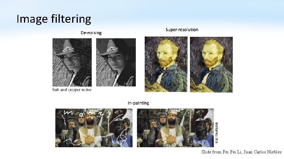
Image filtering • Filtering: • Form a new image whose pixels are a combination of original pixel values. • Goals: • Extract useful information from image • Features (corners, edges, blobs, …) • Enhance image properties • Remove noise, remove unwanted objects, … Slide from Fei Li, Juan Carlos Niebles

Image filtering Slide from Fei Li, Juan Carlos Niebles

Linear filtering: a key idea • Transformations on signals; e. g. : • bass/treble controls on stereo • blurring/sharpening operations in image editing • smoothing/noise reduction in tracking • Key properties • linearity: filter(f + g) = filter(f) + filter(g) • shift invariance: behavior invariant to shifting the input • delaying an audio signal • sliding an image around • Can be modeled mathematically by convolution © 2006 Steve Marschner • 5

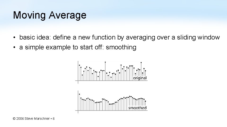
Moving Average • basic idea: define a new function by averaging over a sliding window • a simple example to start off: smoothing © 2006 Steve Marschner • 6

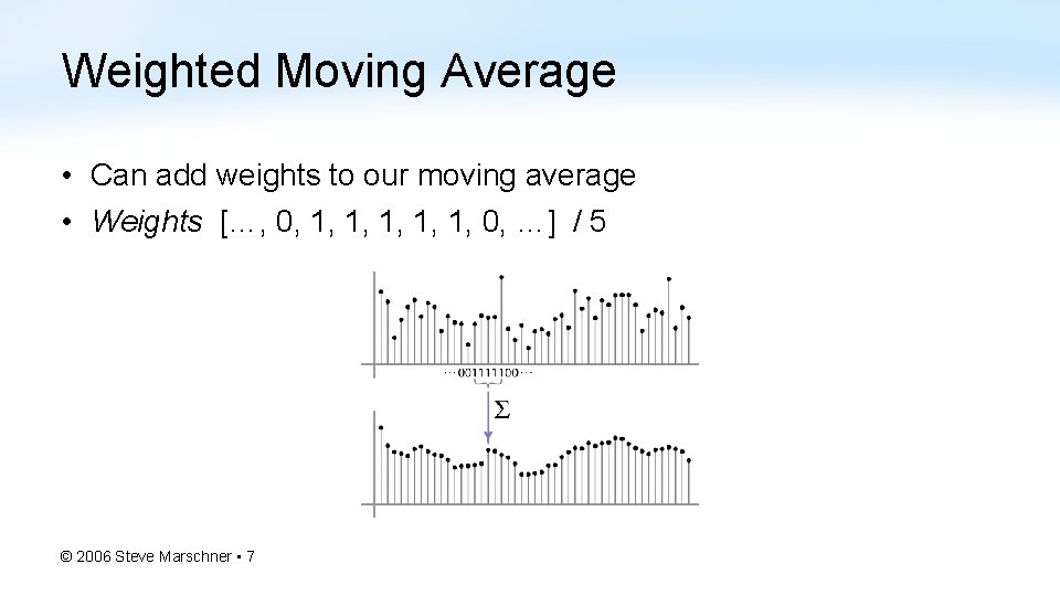
Weighted Moving Average • Can add weights to our moving average • Weights […, 0, 1, 1, 1, 0, …] / 5 © 2006 Steve Marschner • 7

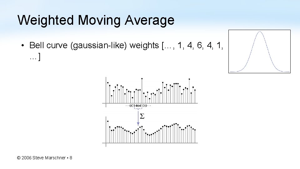
Weighted Moving Average • Bell curve (gaussian-like) weights […, 1, 4, 6, 4, 1, …] © 2006 Steve Marschner • 8

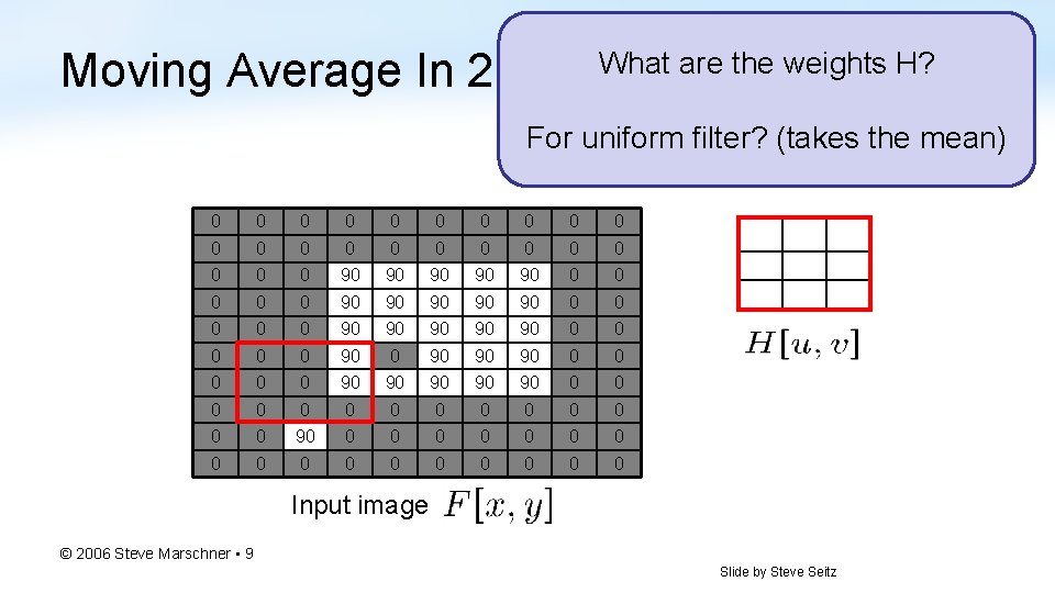
Moving Average In 2 D What are the weights H? For uniform filter? (takes the mean) 0 0 0 0 0 0 90 90 90 0 0 90 90 90 0 90 90 90 0 0 0 0 0 0 0 0 0 0 Input image © 2006 Steve Marschner • 9 Slide by Steve Seitz

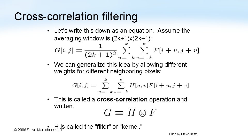
Cross-correlation filtering • Let’s write this down as an equation. Assume the averaging window is (2 k+1)x(2 k+1): • We can generalize this idea by allowing different weights for different neighboring pixels: • This is called a cross-correlation operation and written: • H is called the “filter” or “kernel. ” © 2006 Steve Marschner • 10 Slide by Steve Seitz

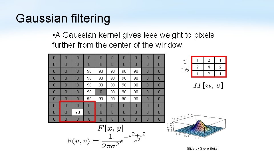
Gaussian filtering • A Gaussian kernel gives less weight to pixels further from the center of the window 0 0 0 0 0 0 90 90 90 0 0 90 90 90 0 90 90 90 0 0 0 0 0 0 0 0 0 0 1 2 4 2 1 Slide by Steve Seitz

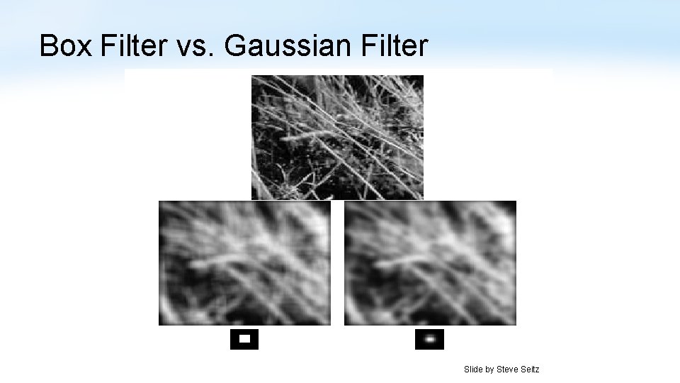
Box Filter vs. Gaussian Filter Slide by Steve Seitz

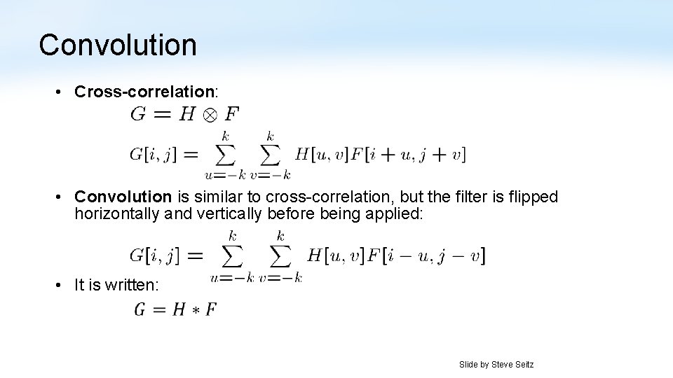
Convolution • Cross-correlation: • Convolution is similar to cross-correlation, but the filter is flipped horizontally and vertically before being applied: • It is written: • Suppose H is a Gaussian or uniform (mean) kernel. How does convolution differ from cross-correlation? Slide by Steve Seitz

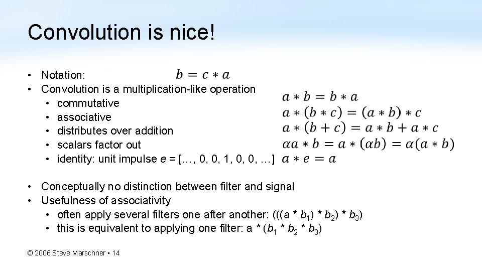
Convolution is nice! • Notation: • Convolution is a multiplication-like operation • commutative • associative • distributes over addition • scalars factor out • identity: unit impulse e = […, 0, 0, 1, 0, 0, …] • Conceptually no distinction between filter and signal • Usefulness of associativity • often apply several filters one after another: (((a * b 1) * b 2) * b 3) • this is equivalent to applying one filter: a * (b 1 * b 2 * b 3) © 2006 Steve Marschner • 14

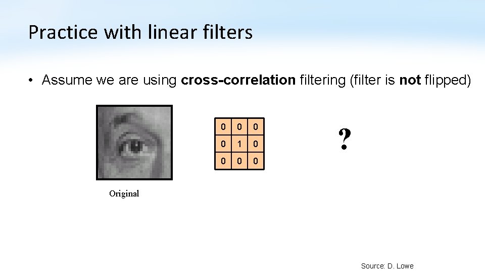
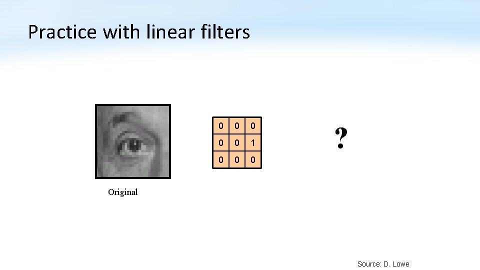
Practice with linear filters • Assume we are using cross-correlation filtering (filter is not flipped) 0 0 1 0 0 ? Original Source: D. Lowe

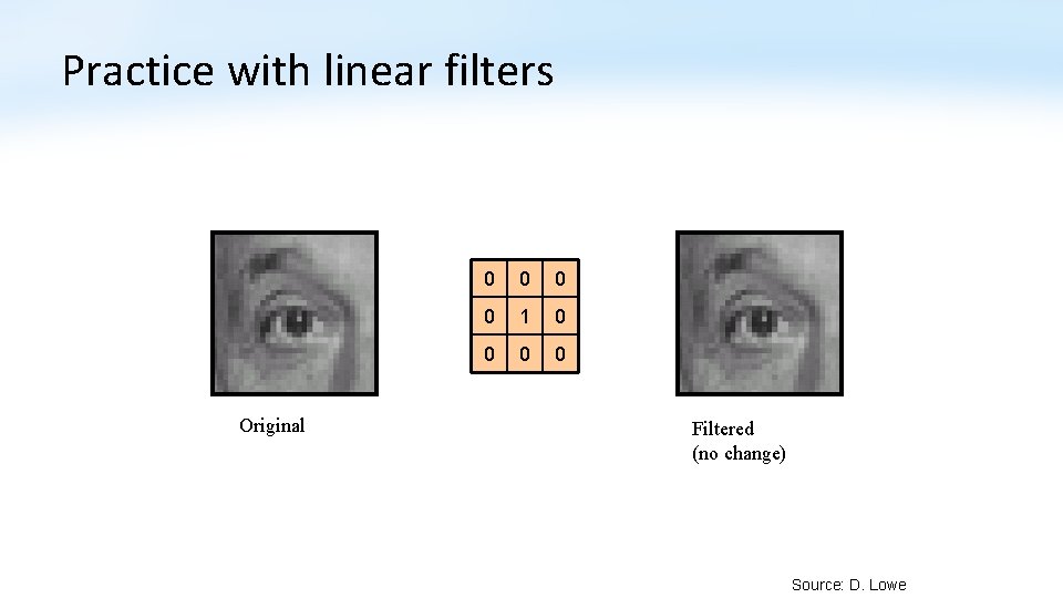
Practice with linear filters Original 0 0 1 0 0 Filtered (no change) Source: D. Lowe

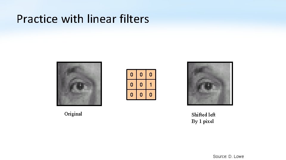
Practice with linear filters 0 0 0 1 0 0 0 ? Original Source: D. Lowe

Practice with linear filters Original 0 0 0 1 0 0 0 Shifted left By 1 pixel Source: D. Lowe

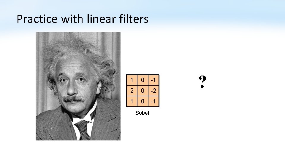
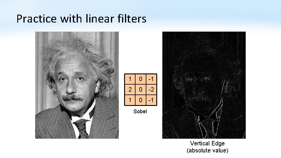
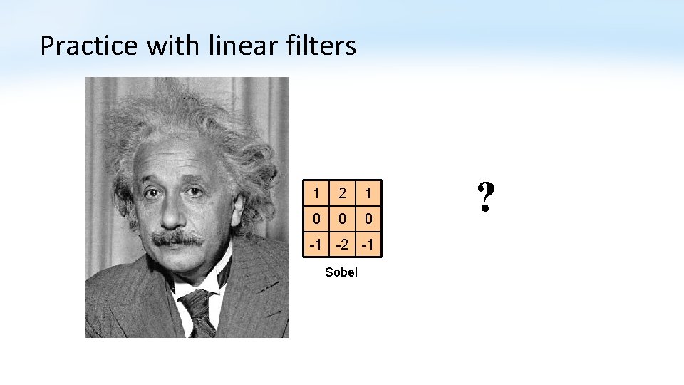
Practice with linear filters 1 0 -1 2 0 -2 1 0 -1 Sobel ?

Practice with linear filters 1 0 -1 2 0 -2 1 0 -1 Sobel Vertical Edge (absolute value)

Practice with linear filters 1 2 1 0 0 0 -1 -2 -1 Sobel ?

Practice with linear filters 1 2 1 0 0 0 -1 -2 -1 Sobel Horizontal Edge (absolute value)

Outline • Filtering • Linear filters: cross-correlation and convolution • Gaussian filters

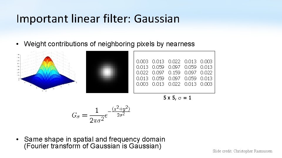
Important linear filter: Gaussian • Weight contributions of neighboring pixels by nearness 0. 003 0. 013 0. 022 0. 013 0. 003 0. 013 0. 059 0. 097 0. 059 0. 013 0. 022 0. 097 0. 159 0. 097 0. 022 0. 013 0. 059 0. 097 0. 059 0. 013 0. 003 0. 013 0. 022 0. 013 0. 003 5 x 5, = 1 • Same shape in spatial and frequency domain (Fourier transform of Gaussian is Gaussian) Slide credit: Christopher Rasmussen

Gaussian filters Input image (2048 x 1397)

Gaussian filters Gaussian filtered (σ=5)

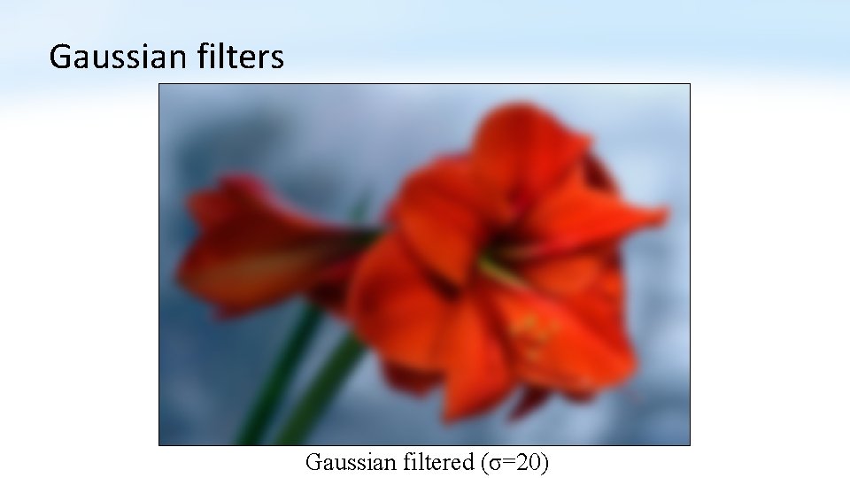
Gaussian filters Gaussian filtered (σ=20)

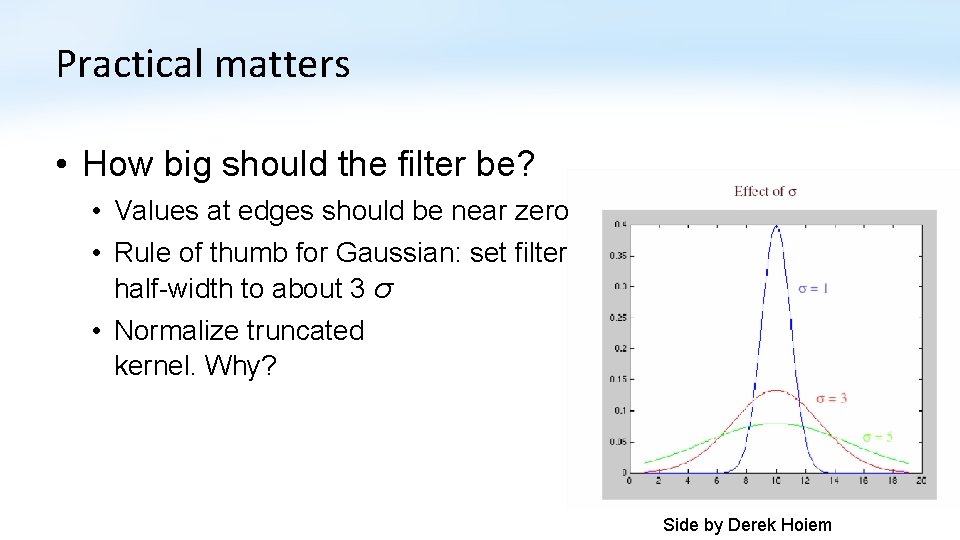
Practical matters • How big should the filter be? • Values at edges should be near zero • Rule of thumb for Gaussian: set filter half-width to about 3 σ • Normalize truncated kernel. Why? Side by Derek Hoiem

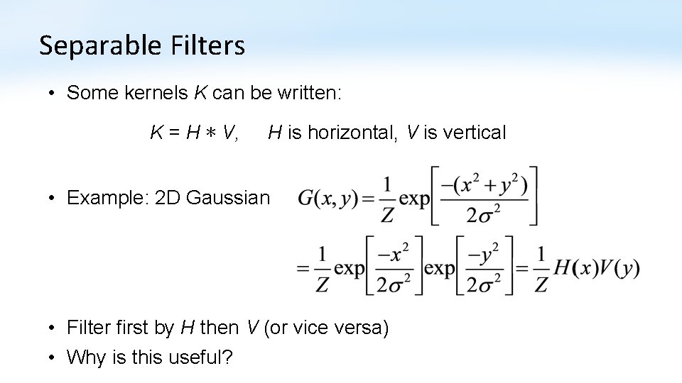
Separable Filters • Some kernels K can be written: K = H ∗ V, H is horizontal, V is vertical • Example: 2 D Gaussian • Filter first by H then V (or vice versa) • Why is this useful?

Filters in Python • scipy. ndimage. filters. convolve • Various pre-defined filters in skimage. filters • Deep Learning libraries (Py. Torch, Tensor. Flow, Keras, …) have efficient GPU convolutions implemented