CS 559 Computer Graphics Lecture 3 Digital Image

CS 559: Computer Graphics Lecture 3: Digital Image Representation Li Zhang Spring 2008

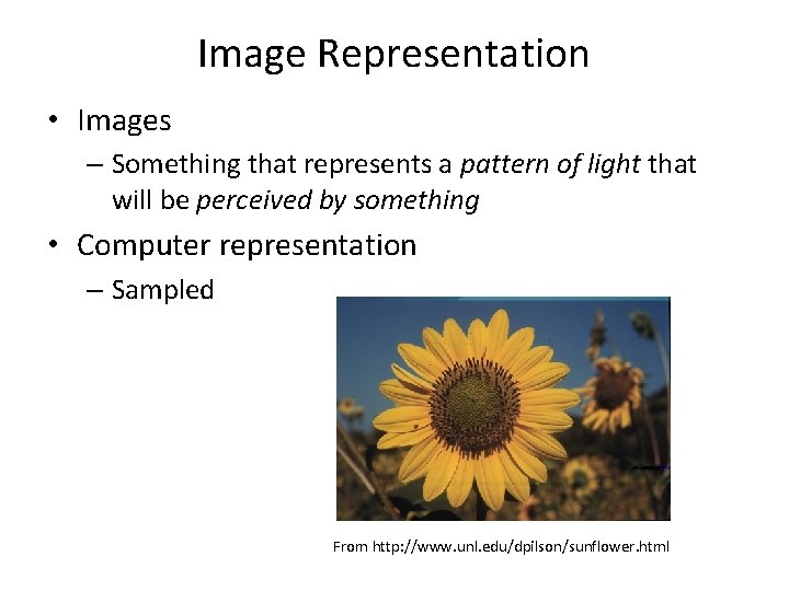
Image Representation • Images – Something that represents a pattern of light that will be perceived by something • Computer representation – Sampled From http: //www. unl. edu/dpilson/sunflower. html

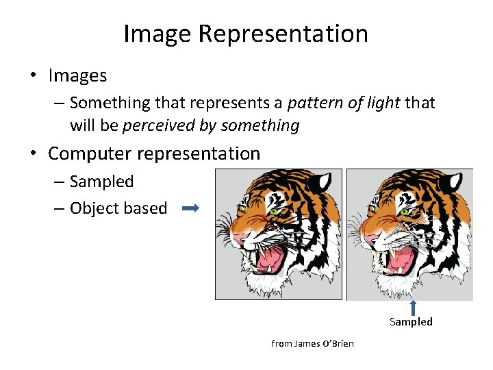
Image Representation • Images – Something that represents a pattern of light that will be perceived by something • Computer representation – Sampled – Object based Sampled from James O’Brien

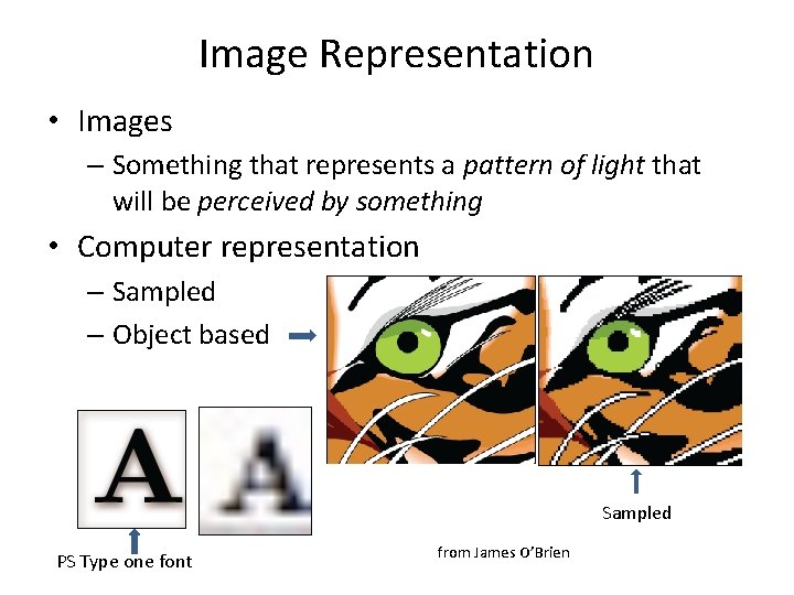
Image Representation • Images – Something that represents a pattern of light that will be perceived by something • Computer representation – Sampled – Object based Sampled PS Type one font from James O’Brien

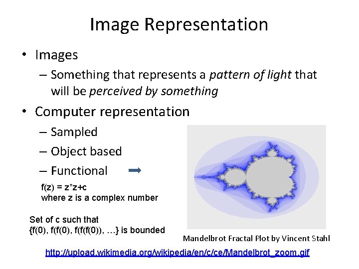
Image Representation • Images – Something that represents a pattern of light that will be perceived by something • Computer representation – Sampled – Object based – Functional f(z) = z*z+c where z is a complex number Set of c such that {f(0), f(f(f(0)), …} is bounded Mandelbrot Fractal Plot by Vincent Stahl http: //upload. wikimedia. org/wikipedia/en/c/ce/Mandelbrot_zoom. gif

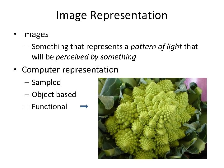
Image Representation • Images – Something that represents a pattern of light that will be perceived by something • Computer representation – Sampled – Object based – Functional

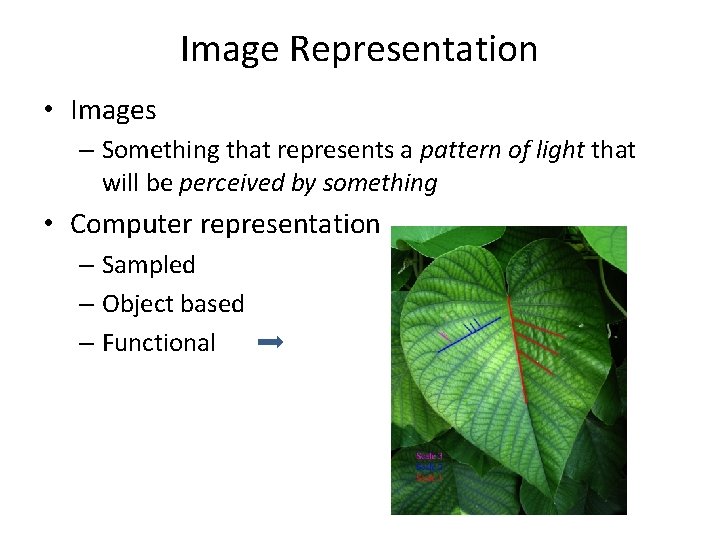
Image Representation • Images – Something that represents a pattern of light that will be perceived by something • Computer representation – Sampled – Object based – Functional

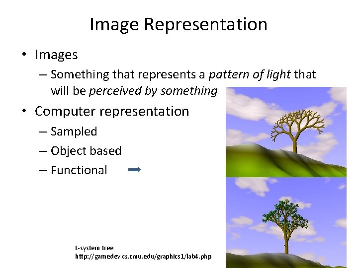
Image Representation • Images – Something that represents a pattern of light that will be perceived by something • Computer representation – Sampled – Object based – Functional L-system tree http: //gamedev. cs. cmu. edu/graphics 1/lab 4. php

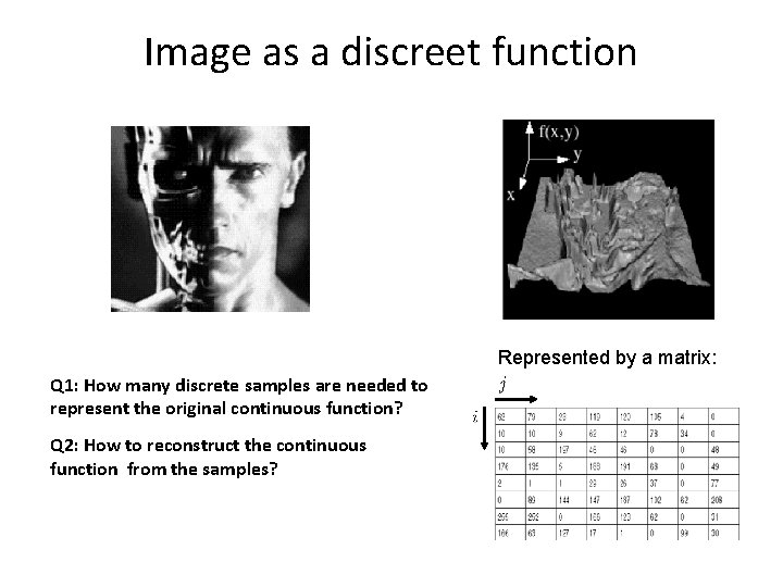
Image as a discreet function Represented by a matrix: Q 1: How many discrete samples are needed to represent the original continuous function? Q 2: How to reconstruct the continuous function from the samples?

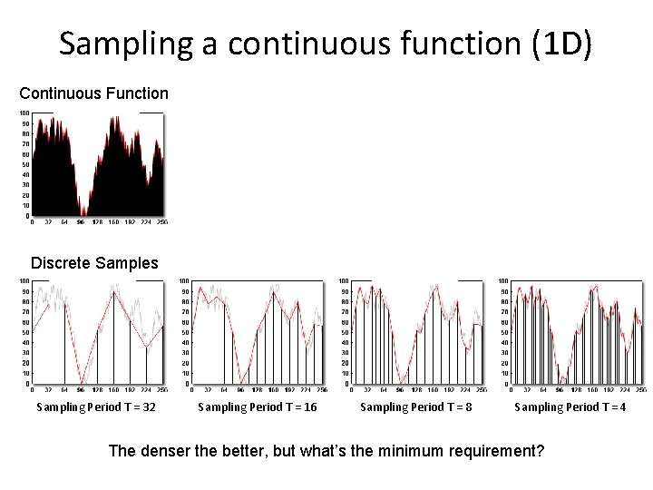
Sampling a continuous function (1 D) Continuous Function Discrete Samples Sampling Period T = 32 Sampling Period T = 16 Sampling Period T = 8 Sampling Period T = 4 The denser the better, but what’s the minimum requirement?

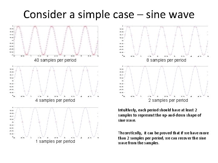
Consider a simple case – sine wave 40 samples period 4 samples period 8 samples period 2 samples period Intuitively, each period should have at least 2 samples to represent the up-and-down shape of sine wave. 1 samples period Theoretically, it can be proved that if we have more than 2 samples period, we can recover the sine wave from the samples.

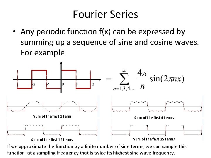
How about general functions? • Idea: represent an arbitrary function using sine waves.

Fourier Series • Any periodic function f(x) can be expressed by summing up a sequence of sine and cosine waves. For example -2 -1 0 1 2 Sum of the first 1 term Sum of the first 4 terms Sum of the first 12 terms Sum of the first 25 terms If we approximate the function by a finite number of sine terms, we can sample this function at a sampling frequency that is twice its highest sine wave frequency.

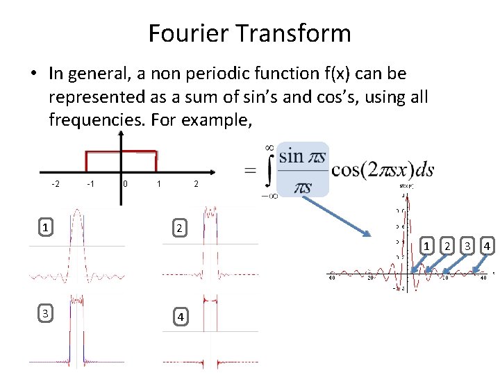
Fourier Transform • In general, a non periodic function f(x) can be represented as a sum of sin’s and cos’s, using all frequencies. For example, -2 1 -1 0 1 2 2 1 3 4 2 3 4

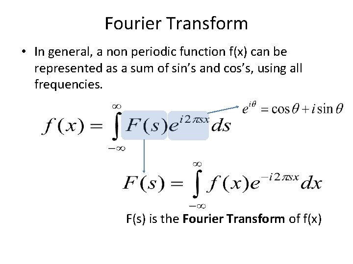
Fourier Transform • In general, a non periodic function f(x) can be represented as a sum of sin’s and cos’s, using all frequencies. F(s) is the Fourier Transform of f(x)

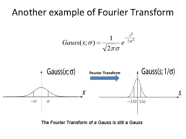
Another example of Fourier Transform -s s -1/s The Fourier Transform of a Gauss is still a Gauss

Sampling theorem • This result is known as the Sampling Theorem and is due to Claude Shannon who first discovered it in 1949: A signal can be reconstructed from its samples without loss of information, if the original signal has no frequencies above ½ the sampling frequency.

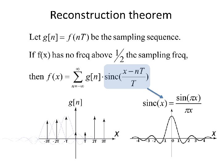
Reconstruction theorem -3 T -2 T -T T 2 T 3 T -4 -3 -2 -1 0 1 2 3 4

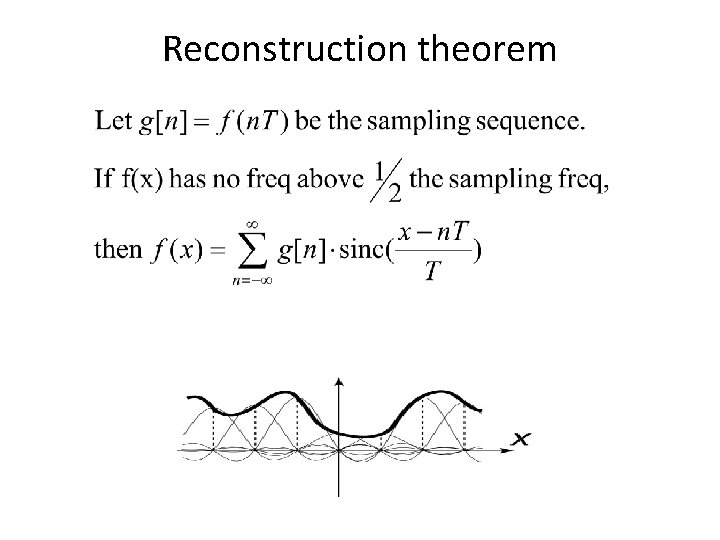
Reconstruction theorem

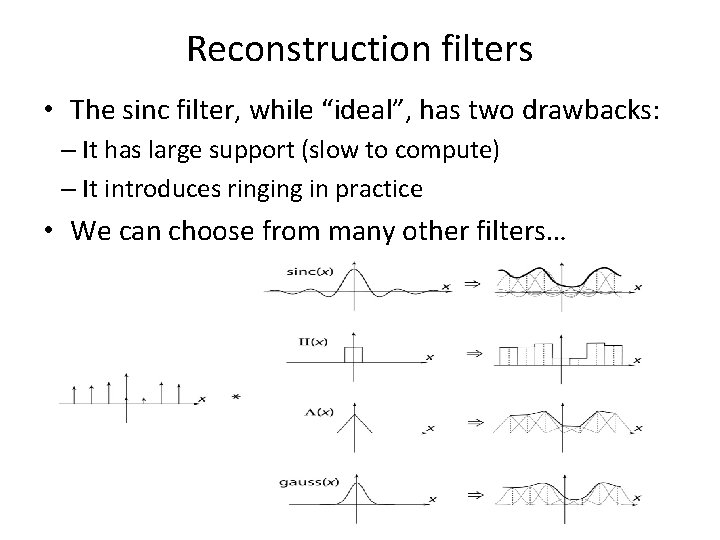
Reconstruction filters • The sinc filter, while “ideal”, has two drawbacks: – It has large support (slow to compute) – It introduces ringing in practice • We can choose from many other filters…

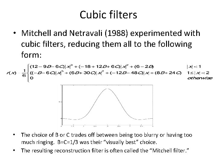
Cubic filters • Mitchell and Netravali (1988) experimented with cubic filters, reducing them all to the following form: • The choice of B or C trades off between being too blurry or having too much ringing. B=C=1/3 was their “visually best” choice. • The resulting reconstruction filter is often called the “Mitchell filter. ”

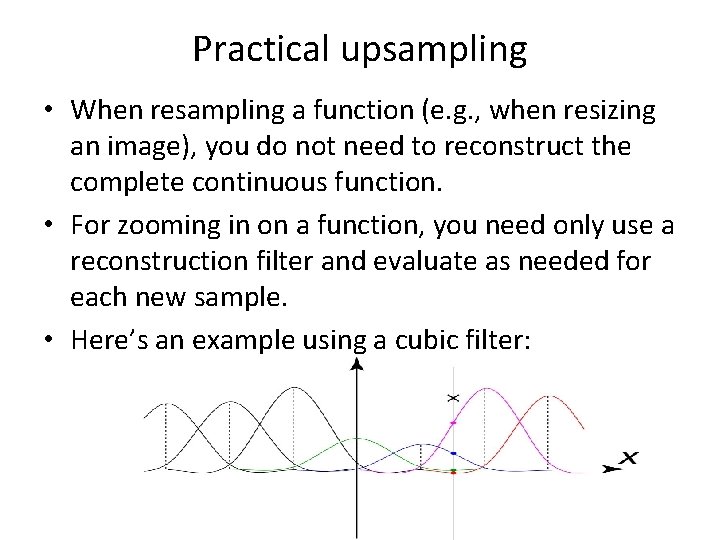
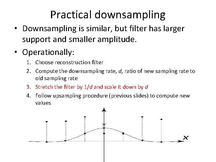
Practical upsampling • When resampling a function (e. g. , when resizing an image), you do not need to reconstruct the complete continuous function. • For zooming in on a function, you need only use a reconstruction filter and evaluate as needed for each new sample. • Here’s an example using a cubic filter:

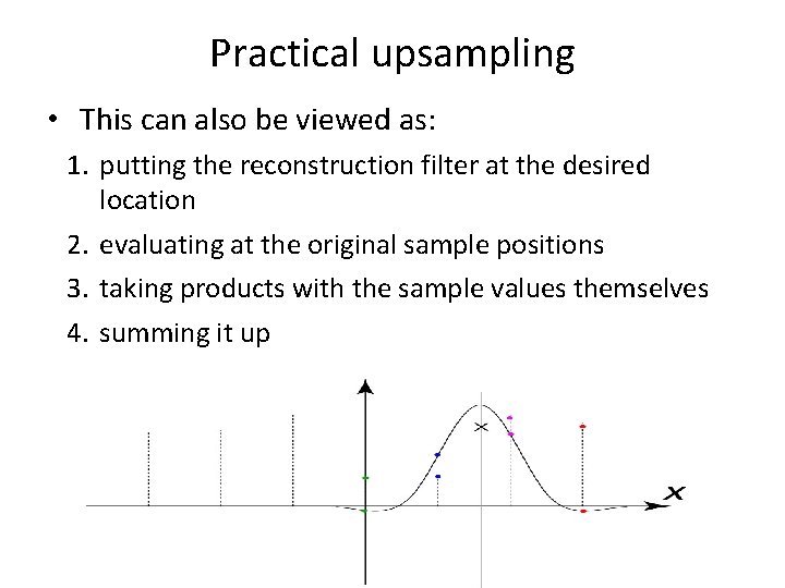
Practical upsampling • This can also be viewed as: 1. putting the reconstruction filter at the desired location 2. evaluating at the original sample positions 3. taking products with the sample values themselves 4. summing it up

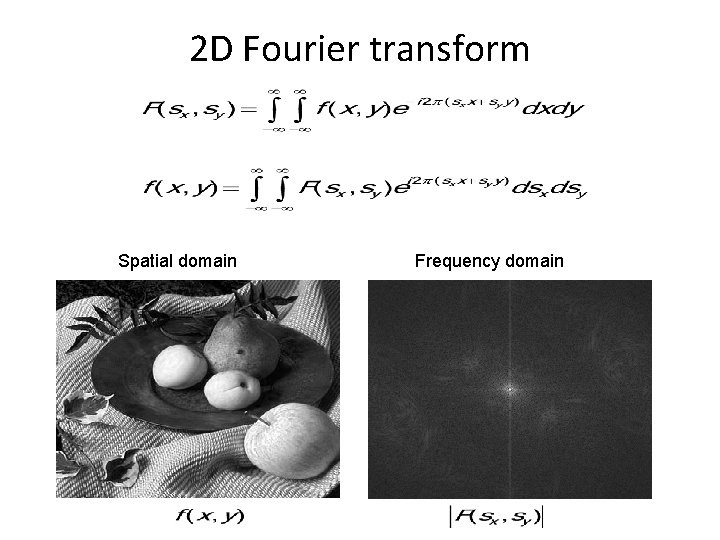
2 D Fourier transform Spatial domain Frequency domain

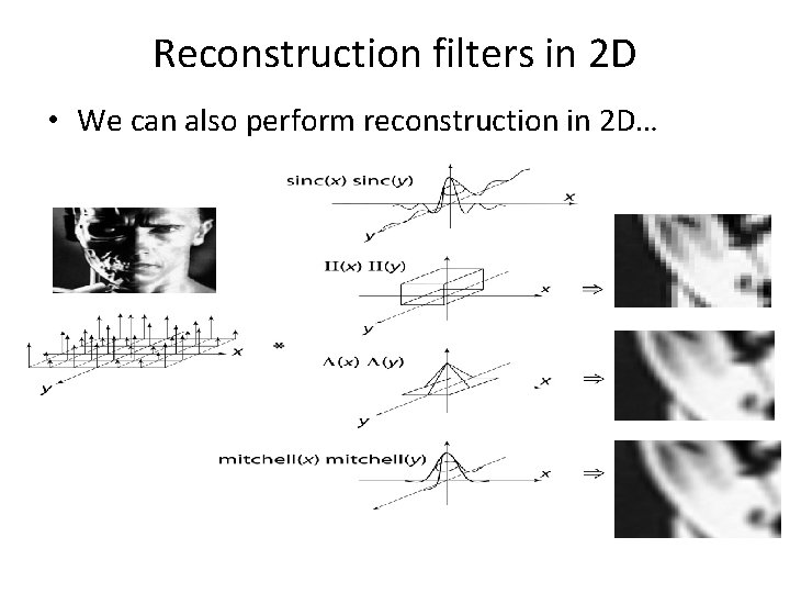
Reconstruction filters in 2 D • We can also perform reconstruction in 2 D…

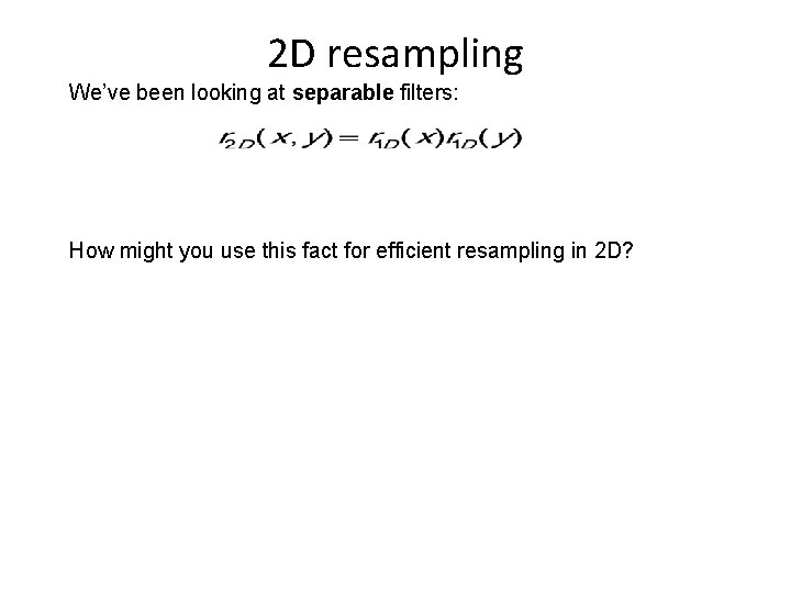
2 D resampling We’ve been looking at separable filters: How might you use this fact for efficient resampling in 2 D?

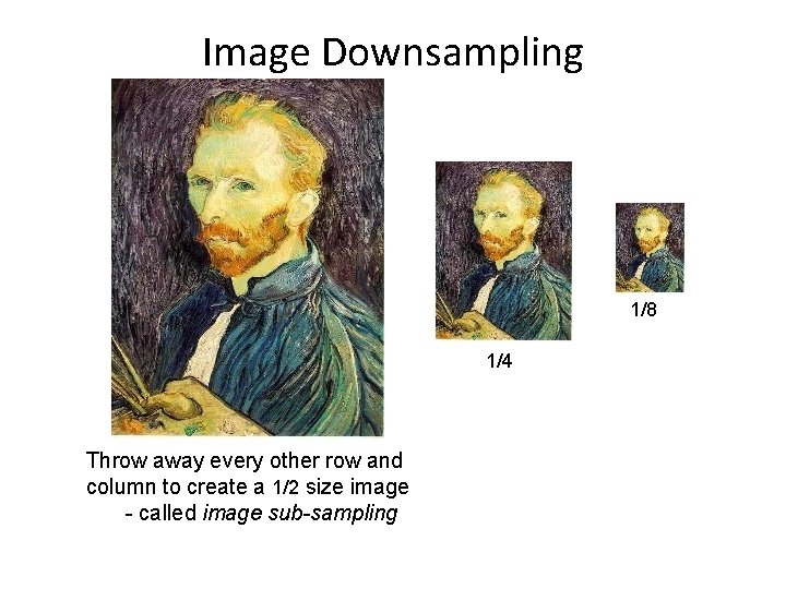
Image Downsampling 1/8 1/4 Throw away every other row and column to create a 1/2 size image - called image sub-sampling

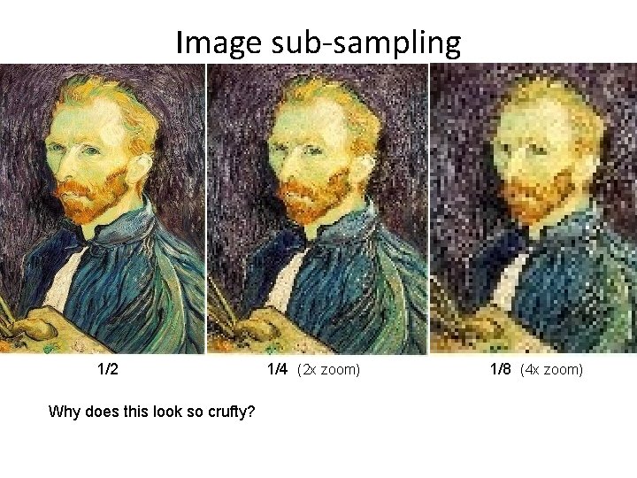
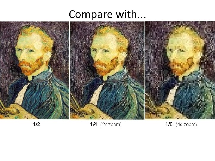
Image sub-sampling 1/2 Why does this look so crufty? 1/4 (2 x zoom) 1/8 (4 x zoom)

Practical downsampling • Downsampling is similar, but filter has larger support and smaller amplitude. • Operationally: 1. Choose reconstruction filter 2. Compute the downsampling rate, d, ratio of new sampling rate to old sampling rate 3. Stretch the filter by 1/d and scale it down by d 4. Follow upsampling procedure (previous slides) to compute new values

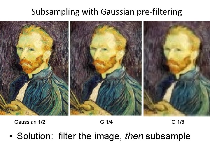
Subsampling with Gaussian pre-filtering Gaussian 1/2 G 1/4 G 1/8 • Solution: filter the image, then subsample

Compare with. . . 1/2 1/4 (2 x zoom) 1/8 (4 x zoom)

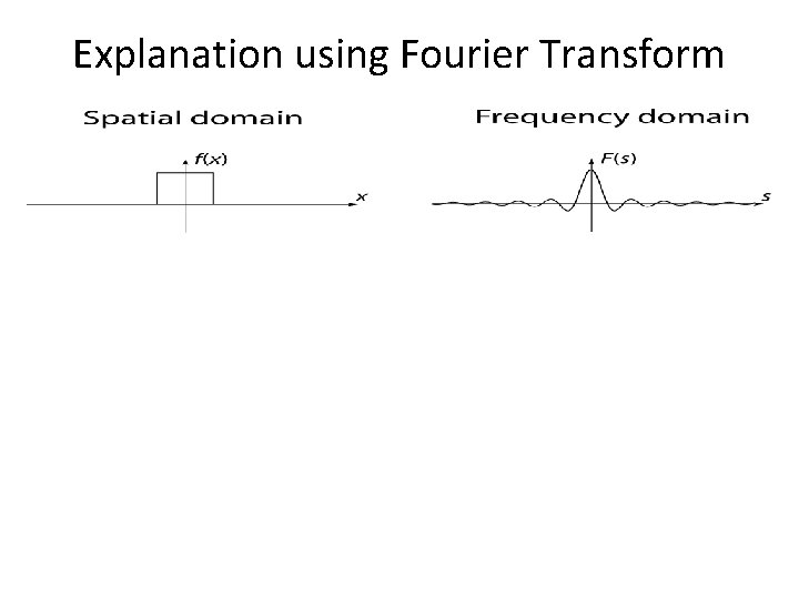
Explanation using Fourier Transform

Explanation using Fourier Transform

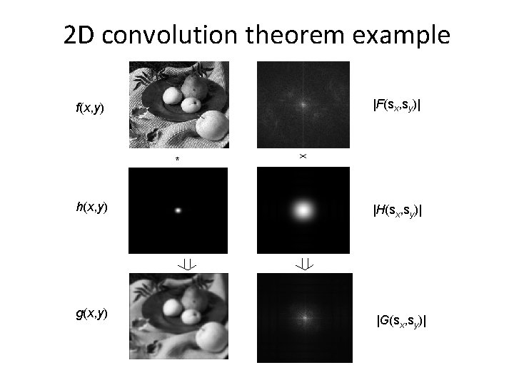
2 D convolution theorem example |F(sx, sy)| f(x, y) * h(x, y) g(x, y) |H(sx, sy)| |G(sx, sy)|

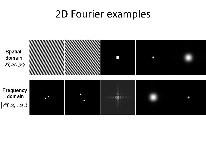
2 D Fourier examples Spatial domain Frequency domain

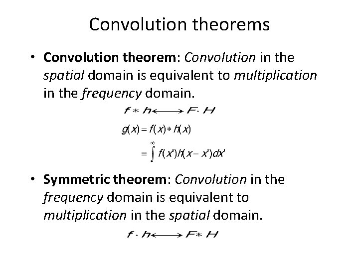
Convolution theorems • Convolution theorem: Convolution in the spatial domain is equivalent to multiplication in the frequency domain. • Symmetric theorem: Convolution in the frequency domain is equivalent to multiplication in the spatial domain.

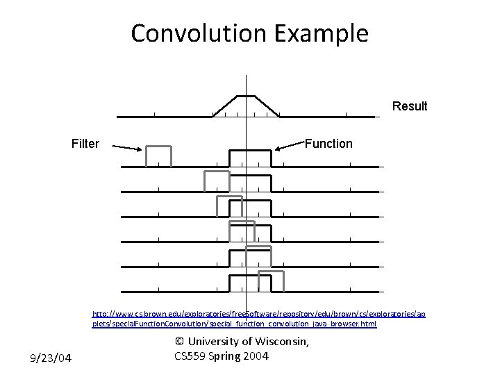
Convolution Example Result Filter Function http: //www. cs. brown. edu/exploratories/free. Software/repository/edu/brown/cs/exploratories/ap plets/special. Function. Convolution/special_function_convolution_java_browser. html 9/23/04 © University of Wisconsin, CS 559 Spring 2004

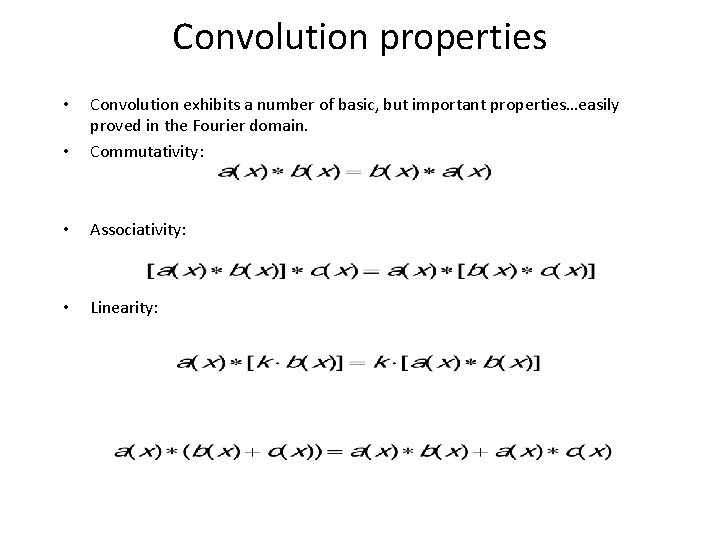
Convolution properties • Convolution exhibits a number of basic, but important properties…easily proved in the Fourier domain. Commutativity: • Associativity: • Linearity: •