CS 559 Computer Graphics Lecture 7 Image Warping

CS 559: Computer Graphics Lecture 7: Image Warping and Panorama Li Zhang Spring 2008 Most slides borrowed from Yungyu Chuang

Today • Image Warping and Morphing • Reading – – Shirley, Ch 5, Linear Algebra Shirley, Ch 6. 1, 2 D Transform Shirley, Ch 6. 3, Translation, p 151 -152(1 st paragraph) (Optional) Image morphing: a survey, George Wolberg, Visual Computer 1998

Image Manipulation • Changing pixel values • Moving pixels around h([x, y])=[x, y/2] f h g

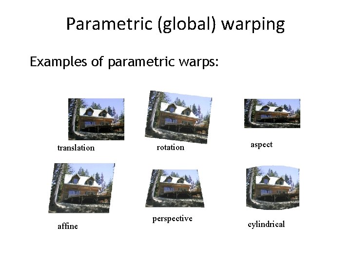
Parametric (global) warping Examples of parametric warps: translation affine rotation perspective aspect cylindrical

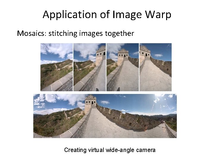
Application of Image Warp Mosaics: stitching images together Creating virtual wide-angle camera

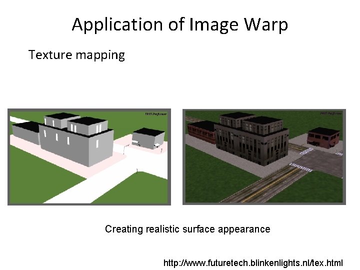
Application of Image Warp Texture mapping Creating realistic surface appearance http: //www. futuretech. blinkenlights. nl/tex. html

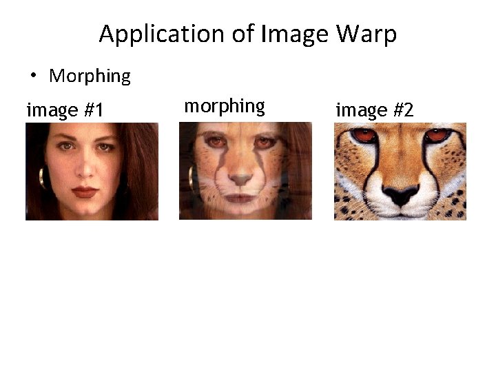
Application of Image Warp • Morphing image #1 morphing image #2

Parametric (global) warping h([x, y])=[x, y/2] T p = (x, y) p’ = (x’, y’) • Transformation T is a coordinate-changing machine: p’ = T(p) • What does it mean that T is global? – can be described by just a few numbers (parameters) – the parameters are the same for any point p • Represent T as a matrix: p’ = Mp

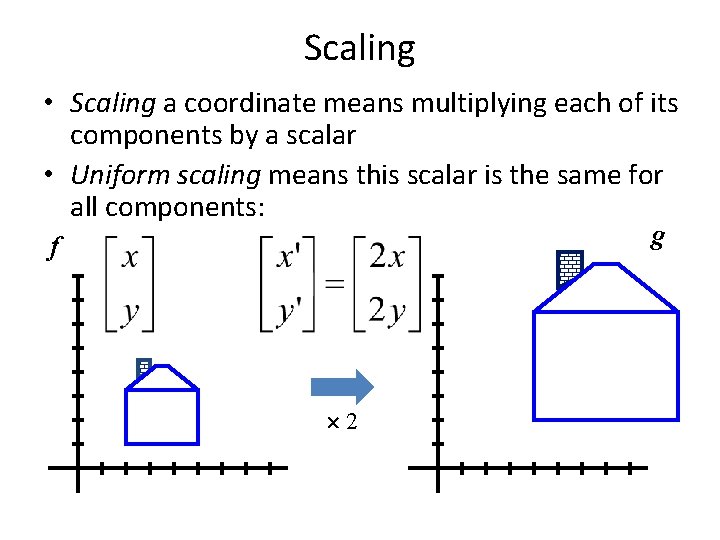
Scaling • Scaling a coordinate means multiplying each of its components by a scalar • Uniform scaling means this scalar is the same for all components: g f 2

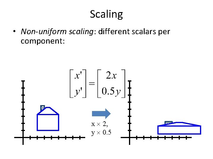
Scaling • Non-uniform scaling: different scalars per component: x 2, y 0. 5

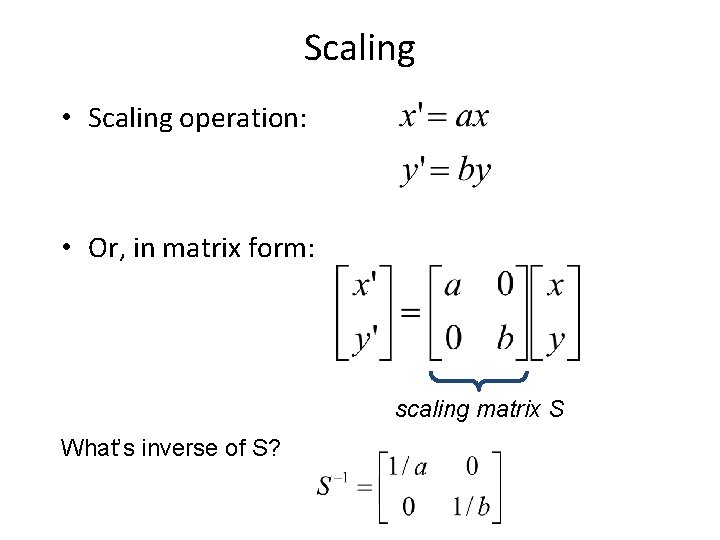
Scaling • Scaling operation: • Or, in matrix form: scaling matrix S What’s inverse of S?

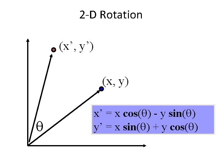
2 -D Rotation (x’, y’) (x, y) x’ = x cos( ) - y sin( ) y’ = x sin( ) + y cos( )

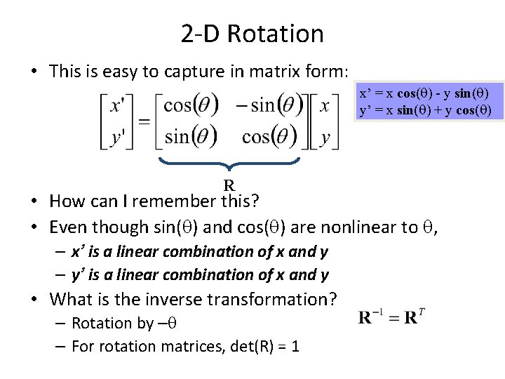
2 -D Rotation • This is easy to capture in matrix form: x’ = x cos( ) - y sin( ) y’ = x sin( ) + y cos( ) R • How can I remember this? • Even though sin( ) and cos( ) are nonlinear to , – x’ is a linear combination of x and y – y’ is a linear combination of x and y • What is the inverse transformation? – Rotation by – – For rotation matrices, det(R) = 1

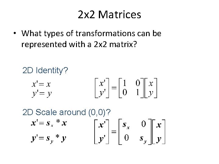
2 x 2 Matrices • What types of transformations can be represented with a 2 x 2 matrix? 2 D Identity? 2 D Scale around (0, 0)?

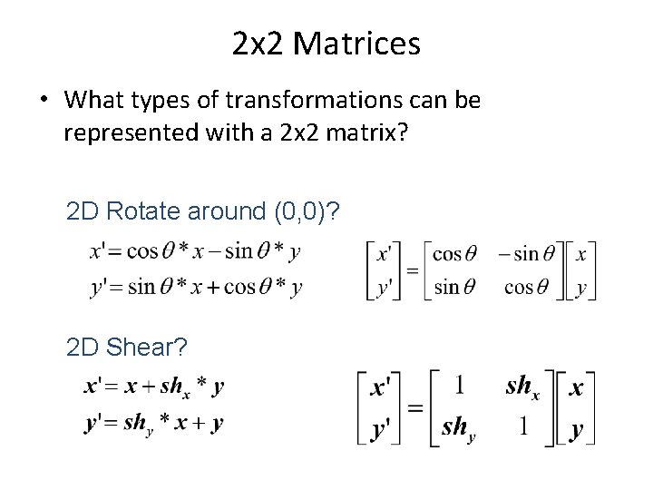
2 x 2 Matrices • What types of transformations can be represented with a 2 x 2 matrix? 2 D Rotate around (0, 0)? 2 D Shear?

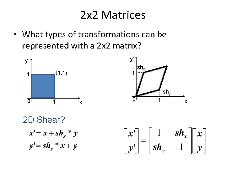
2 x 2 Matrices • What types of transformations can be represented with a 2 x 2 matrix? y’ y 1 1 (1, 1) shx shy 0 1 2 D Shear? x 0 1 x’

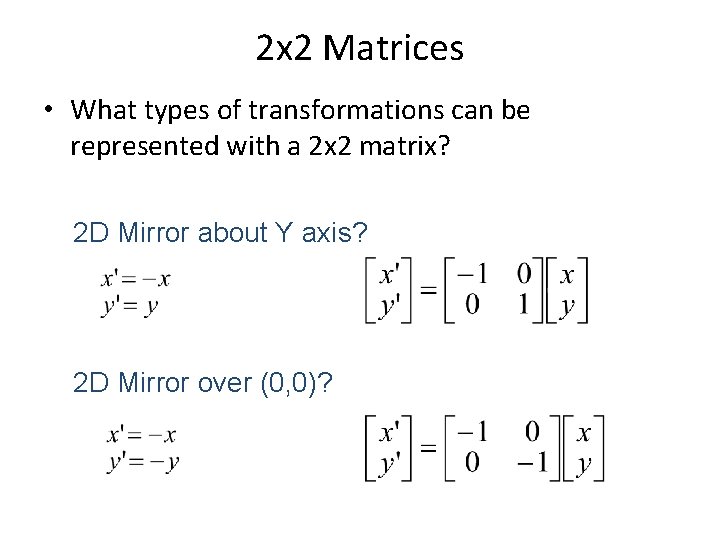
2 x 2 Matrices • What types of transformations can be represented with a 2 x 2 matrix? 2 D Mirror about Y axis? 2 D Mirror over (0, 0)?

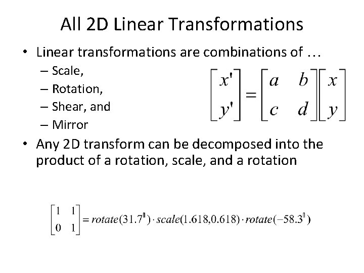
All 2 D Linear Transformations • Linear transformations are combinations of … – Scale, – Rotation, – Shear, and – Mirror • Any 2 D transform can be decomposed into the product of a rotation, scale, and a rotation

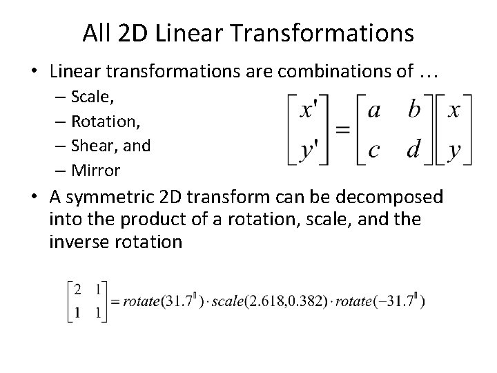
All 2 D Linear Transformations • Linear transformations are combinations of … – Scale, – Rotation, – Shear, and – Mirror • A symmetric 2 D transform can be decomposed into the product of a rotation, scale, and the inverse rotation

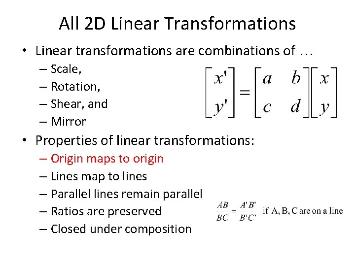
All 2 D Linear Transformations • Linear transformations are combinations of … – Scale, – Rotation, – Shear, and – Mirror • Properties of linear transformations: – Origin maps to origin – Lines map to lines – Parallel lines remain parallel – Ratios are preserved – Closed under composition

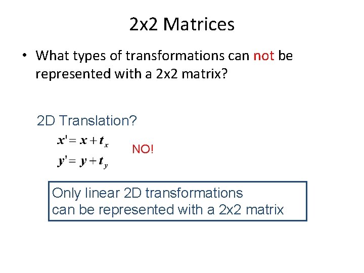
2 x 2 Matrices • What types of transformations can not be represented with a 2 x 2 matrix? 2 D Translation? NO! Only linear 2 D transformations can be represented with a 2 x 2 matrix

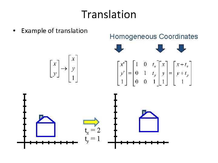
Translation • Example of translation tx = 2 ty = 1 Homogeneous Coordinates

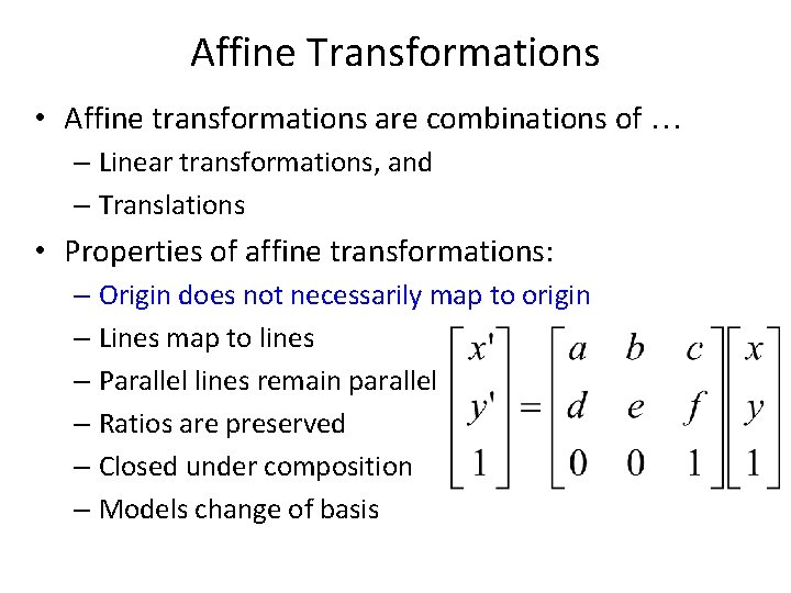
Affine Transformations • Affine transformations are combinations of … – Linear transformations, and – Translations • Properties of affine transformations: – Origin does not necessarily map to origin – Lines map to lines – Parallel lines remain parallel – Ratios are preserved – Closed under composition – Models change of basis

Image warping • Given a coordinate transform x’ = T(x) and a source image I(x), how do we compute a transformed image I’(x’) = I(T(x))? T(x) x I(x) x’ I’(x’)

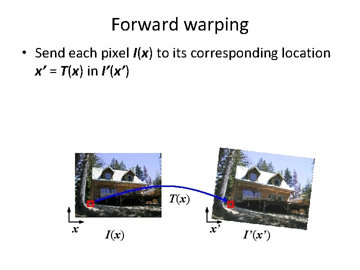
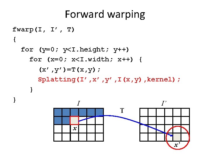
Forward warping • Send each pixel I(x) to its corresponding location x’ = T(x) in I’(x’) T(x) x I(x) x’ I’(x’)

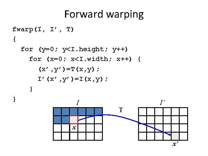
Forward warping fwarp(I, I’, T) { for (y=0; y<I. height; y++) for (x=0; x<I. width; x++) { (x’, y’)=T(x, y); I’(x’, y’)=I(x, y); } } I T I’ x x’

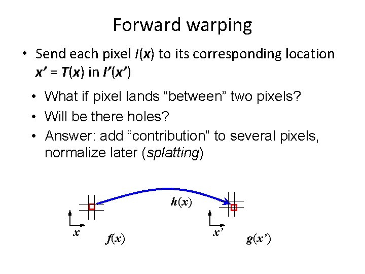
Forward warping • Send each pixel I(x) to its corresponding location x’ = T(x) in I’(x’) • What if pixel lands “between” two pixels? • Will be there holes? • Answer: add “contribution” to several pixels, normalize later (splatting) h(x) x f(x) x’ g(x’)

Forward warping fwarp(I, I’, T) { for (y=0; y<I. height; y++) for (x=0; x<I. width; x++) { (x’, y’)=T(x, y); Splatting(I’, x’, y’, I(x, y), kernel); } } I I’ T x x’

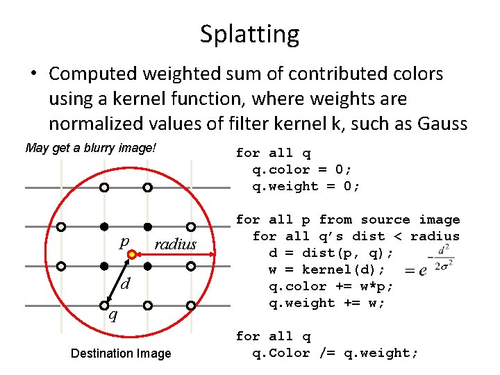
Splatting • Computed weighted sum of contributed colors using a kernel function, where weights are normalized values of filter kernel k, such as Gauss May get a blurry image! p radius d q Destination Image for all q q. color = 0; q. weight = 0; for all p from source image for all q’s dist < radius d = dist(p, q); w = kernel(d); q. color += w*p; q. weight += w; for all q q. Color /= q. weight;

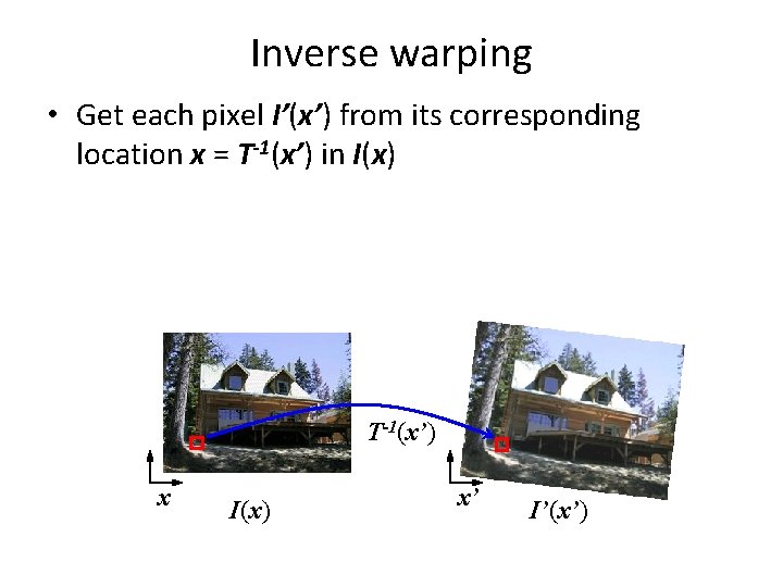
Inverse warping • Get each pixel I’(x’) from its corresponding location x = T-1(x’) in I(x) T-1(x’) x I(x) x’ I’(x’)

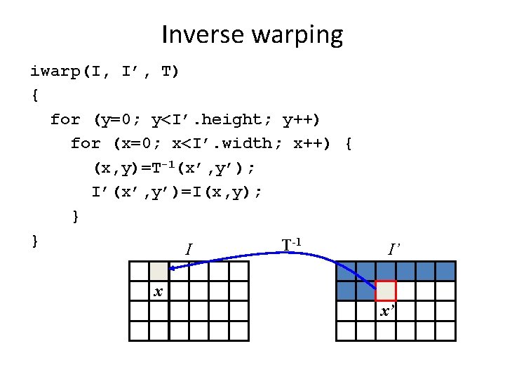
Inverse warping iwarp(I, I’, T) { for (y=0; y<I’. height; y++) for (x=0; x<I’. width; x++) { (x, y)=T-1(x’, y’); I’(x’, y’)=I(x, y); } } T-1 I I’ x x’

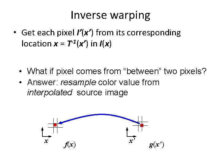
Inverse warping • Get each pixel I’(x’) from its corresponding location x = T-1(x’) in I(x) • What if pixel comes from “between” two pixels? • Answer: resample color value from interpolated source image x f(x) x’ g(x’)

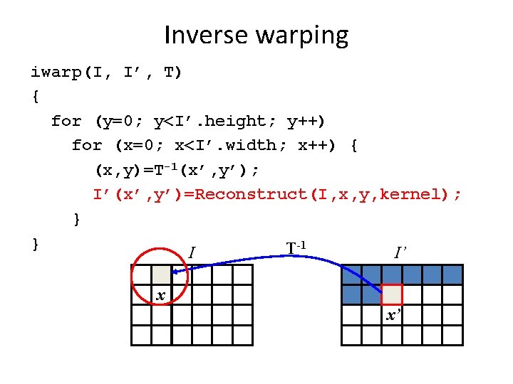
Inverse warping iwarp(I, I’, T) { for (y=0; y<I’. height; y++) for (x=0; x<I’. width; x++) { (x, y)=T-1(x’, y’); I’(x’, y’)=Reconstruct(I, x, y, kernel); } } T-1 I I’ x x’

Reconstruction (interpolation) • Possible reconstruction filters (kernels): – nearest neighbor – bilinear – bicubic – sinc

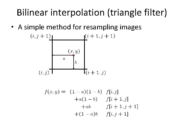
Bilinear interpolation (triangle filter) • A simple method for resampling images

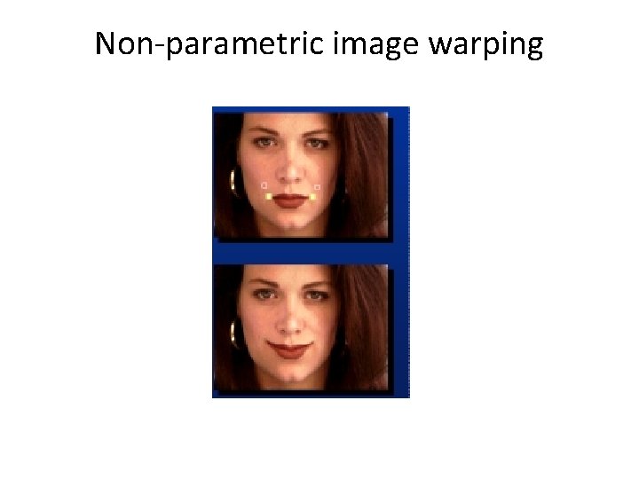
Non-parametric image warping

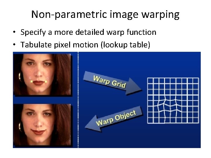
Non-parametric image warping • Specify a more detailed warp function [x, y] T [x’, y’]

Non-parametric image warping • Specify a more detailed warp function • Tabulate pixel motion (lookup table)

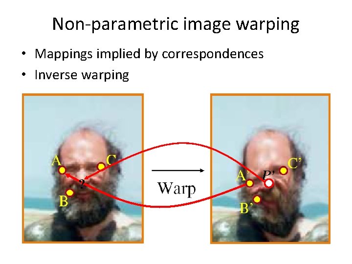
Non-parametric image warping • Mappings implied by correspondences • Inverse warping ? P’

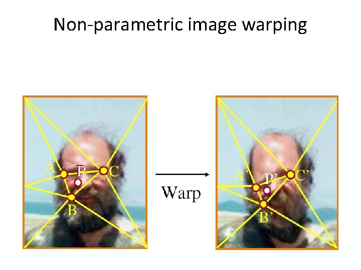
Non-parametric image warping

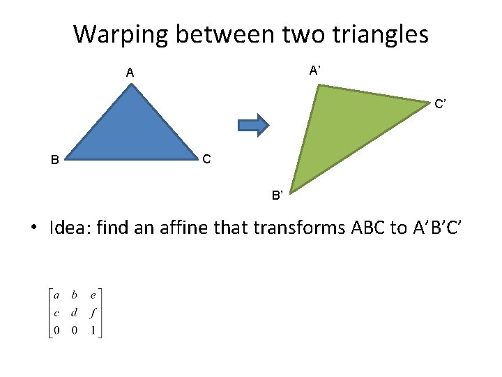
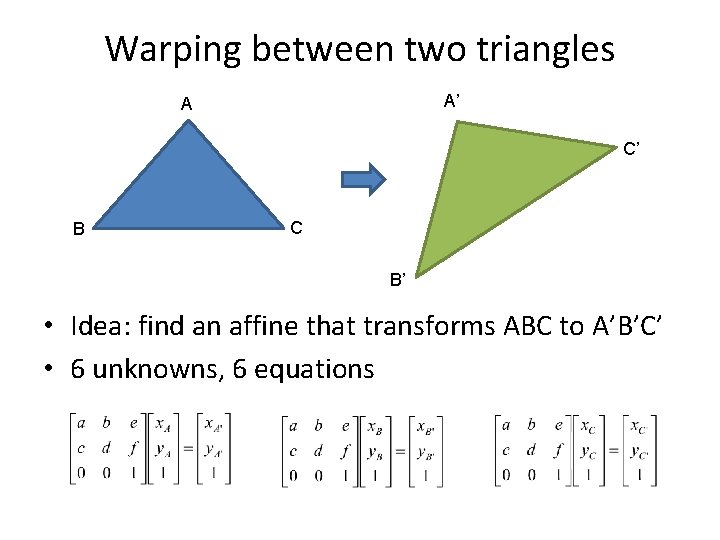
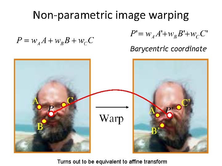
Warping between two triangles A’ A C’ B C B’ • Idea: find an affine that transforms ABC to A’B’C’

Warping between two triangles A’ A C’ B C B’ • Idea: find an affine that transforms ABC to A’B’C’ • 6 unknowns, 6 equations

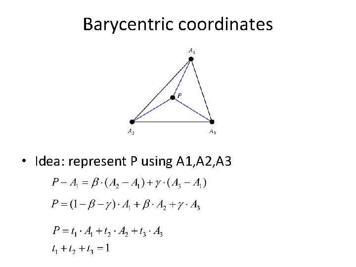
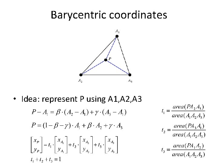
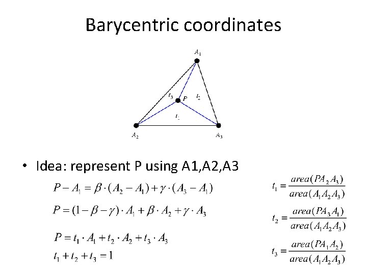
Barycentric coordinates • Idea: represent P using A 1, A 2, A 3

Barycentric coordinates • Idea: represent P using A 1, A 2, A 3

Barycentric coordinates • Idea: represent P using A 1, A 2, A 3

Non-parametric image warping Barycentric coordinate P P’ Turns out to be equivalent to affine transform

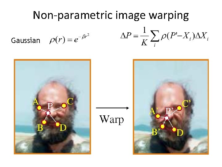
Non-parametric image warping Gaussian

Demo • http: //www. colonize. com/warp 04 -2. php • Warping is a useful operation for mosaics, video matching, view interpolation and so on.

Image morphing

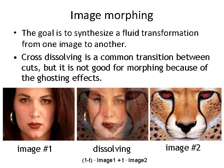
Image morphing • The goal is to synthesize a fluid transformation from one image to another. • Cross dissolving is a common transition between cuts, but it is not good for morphing because of the ghosting effects. image #1 dissolving (1 -t) ∙ Image 1 + t ∙ Image 2 image #2

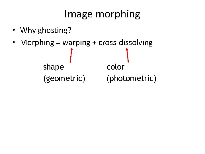
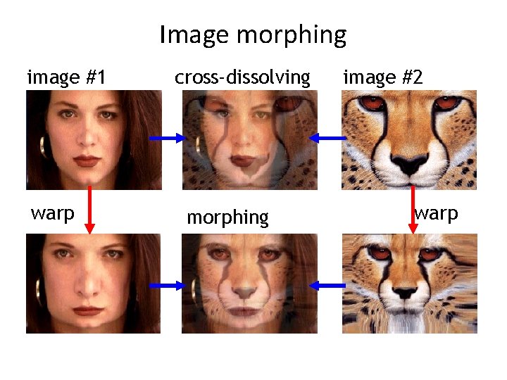
Image morphing • Why ghosting? • Morphing = warping + cross-dissolving shape (geometric) color (photometric)

Image morphing image #1 warp cross-dissolving morphing image #2 warp

Morphing sequence

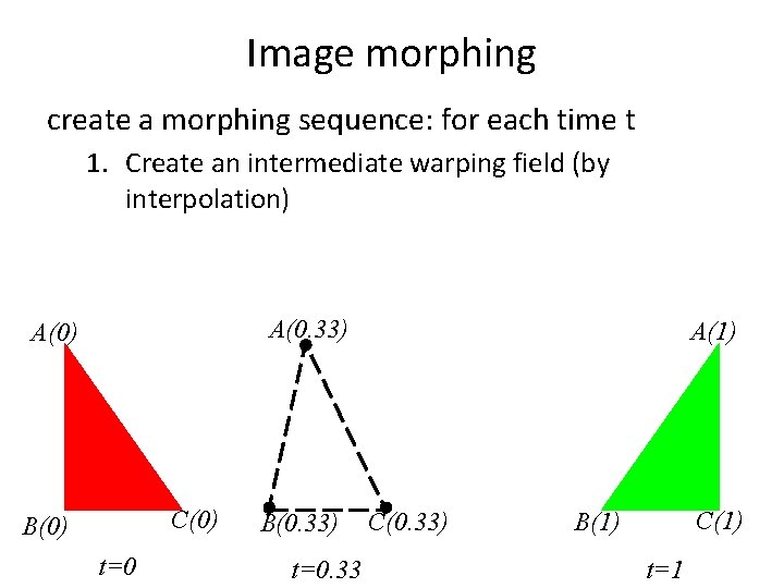
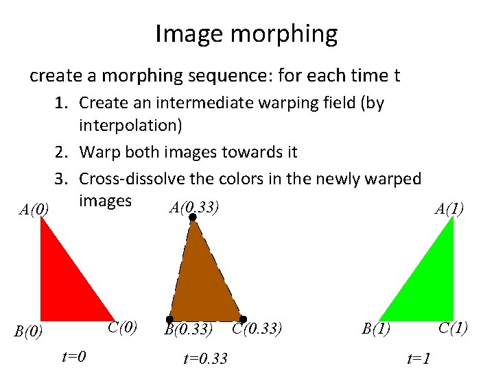
Image morphing create a morphing sequence: for each time t 1. Create an intermediate warping field (by interpolation) A(0. 33) A(0) C(0) B(0) t=0 B(0. 33) t=0. 33 A(1) C(0. 33) C(1) B(1) t=1

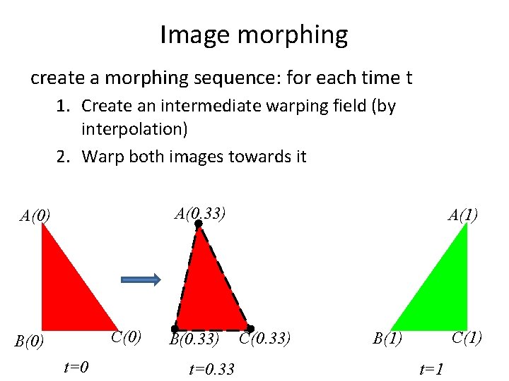
Image morphing create a morphing sequence: for each time t 1. Create an intermediate warping field (by interpolation) 2. Warp both images towards it A(0. 33) A(0) C(0) B(0) t=0 B(0. 33) t=0. 33 A(1) C(0. 33) C(1) B(1) t=1

Image morphing create a morphing sequence: for each time t 1. Create an intermediate warping field (by interpolation) 2. Warp both images towards it A(0. 33) A(0) C(0) B(0) t=0 B(0. 33) t=0. 33 A(1) C(0. 33) C(1) B(1) t=1

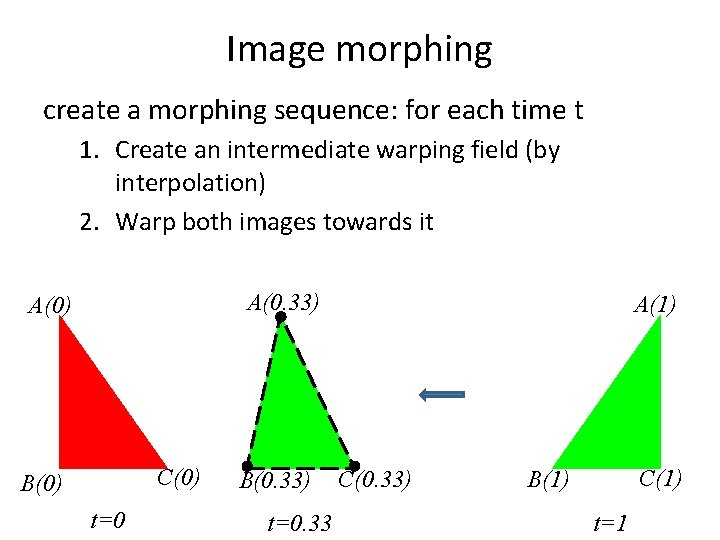
Image morphing create a morphing sequence: for each time t 1. Create an intermediate warping field (by interpolation) 2. Warp both images towards it 3. Cross-dissolve the colors in the newly warped images A(0. 33) A(1) A(0) C(0) B(0) t=0 B(0. 33) t=0. 33 C(0. 33) C(1) B(1) t=1

More complex morph • Triangular Mesh

Results Michael Jackson’s MTV “Black or White” http: //www. michaeljackson. com/quicktime_blackorwhite. html

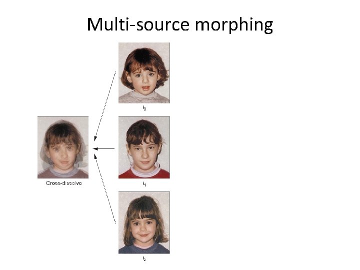
Multi-source morphing

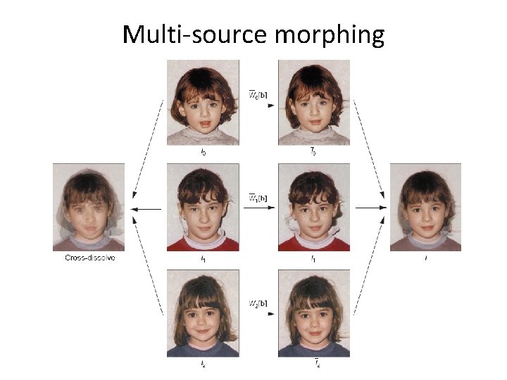
Multi-source morphing

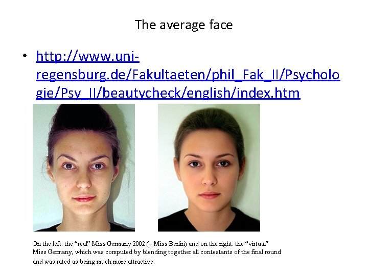
The average face • http: //www. uniregensburg. de/Fakultaeten/phil_Fak_II/Psycholo gie/Psy_II/beautycheck/english/index. htm

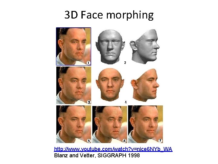
3 D Face morphing http: //www. youtube. com/watch? v=nice 6 NYb_WA Blanz and Vetter, SIGGRAPH 1998