CS 559 Computer Graphics Lecture 4 Image Filtering

CS 559: Computer Graphics Lecture 4: Image Filtering and Resampling Li Zhang Spring 2010

Announcement • Feb 3 rd (this Wed) office hour moves to 4. 305. 30 pm due to CS Department Faculty meeting 3. 30 -4. 30.

Last time: Image Sampling and Filtering Continuous Function Discrete Samples Sampling Period T = 32 Sampling Period T = 16 Sampling Period T = 8 Sampling Period T = 4 The denser the better, but at the expense of storage and processing power

Under-sampling • Sampling a sine wave Some information loss Ambiguous signal interpretation

Under-sampling • Sampling a sine wave Some information loss Ambiguous signal interpretation

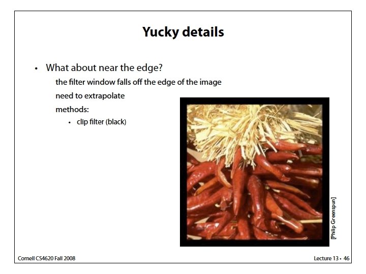
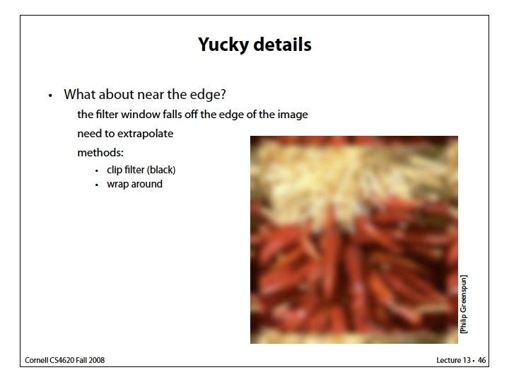
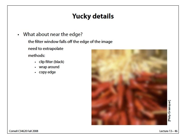
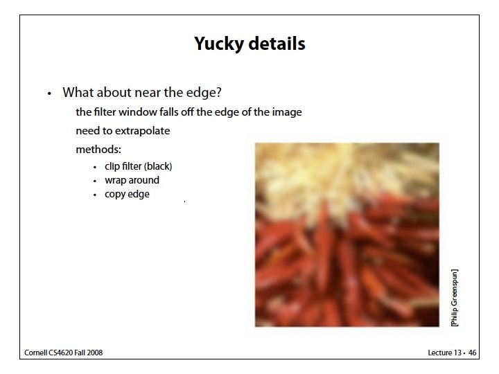
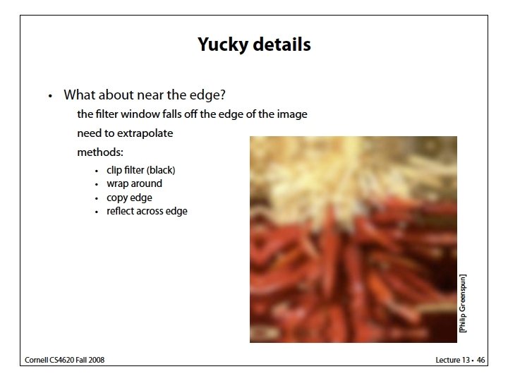
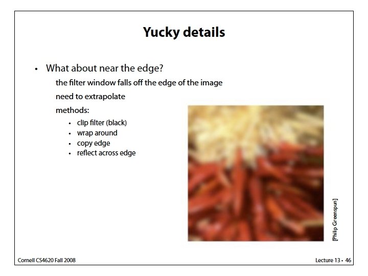
Preventing aliasing Introducing lowpass filters: remove high frequency leaving only safe low frequencies choose lowest frequency in reconstruction (disambiguate)

Assuming zero padding outside the nonzero filter support

a 0 0 0. 5 0 0 a

Sharpening by Filtering before after

The filter can have rectangular shape as well. For example 3 x 5.

The filter can have rectangular shape as well. For example 3 x 5. 0 1 0 0 2 0 0 1 0

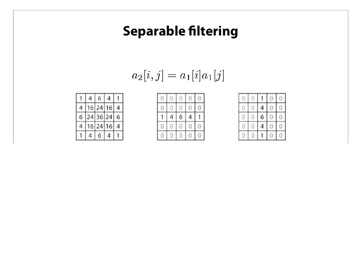
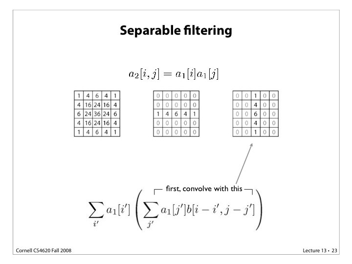
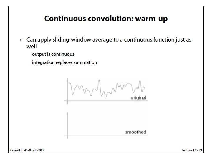
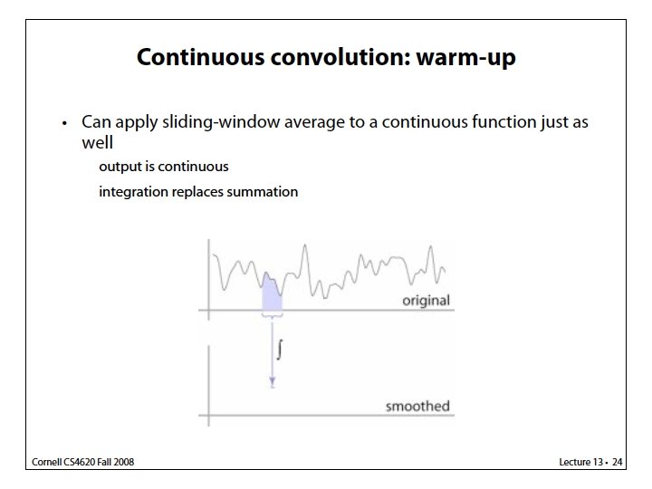
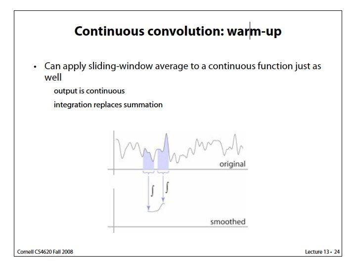
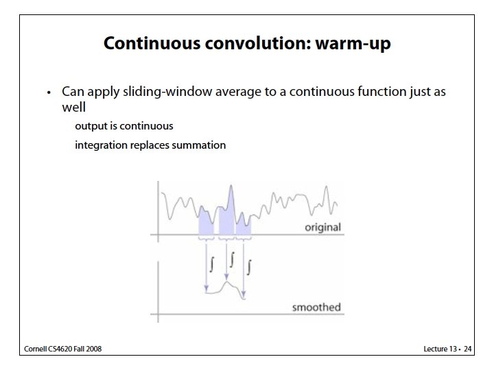
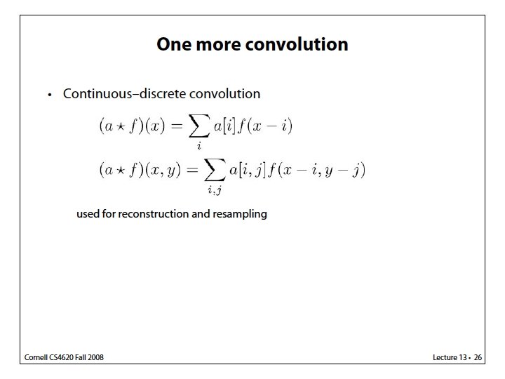
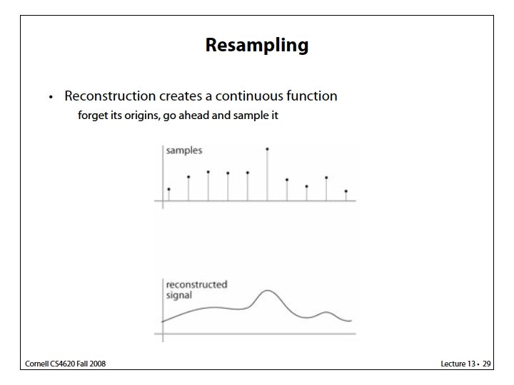
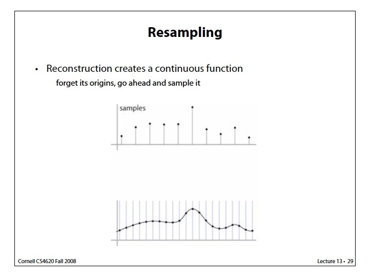
Today’s topics • Continuous Convolution • Continuous-discrete convolution • Resampling

Let’s do a concrete example

Delta Function • The counterpart of convolution 0 0 1 0 0 for continuous

Delta Function • The counterpart of convolution • (δ★ f)(x)=f(x) 0 0 1 0 0 for continuous

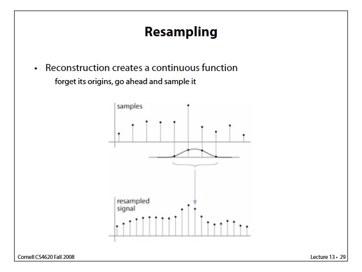
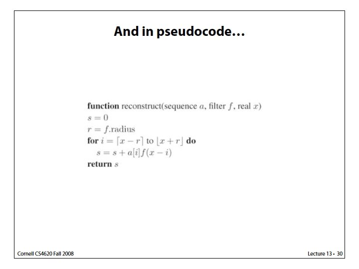
1. 2. 3. 4. putting the flipped reconstruction filter at the desired location evaluating at the original sample positions taking products with the sample values themselves summing it up

1. 2. 3. 4. putting the flipped reconstruction filter at the desired location evaluating at the original sample positions taking products with the sample values themselves summing it up

Another view on continuous-discrete convolution Reconstruction (discrete-continuous convolution) as a sum of shifted copies of the filter Same view also holds for discrete convolution

An Example:

An Example:

Let’s take a break

Discontinuous Reconstruction

How to use box filter • Method 1 • Method 2

How to use tent filter • Method 1 • Method 2

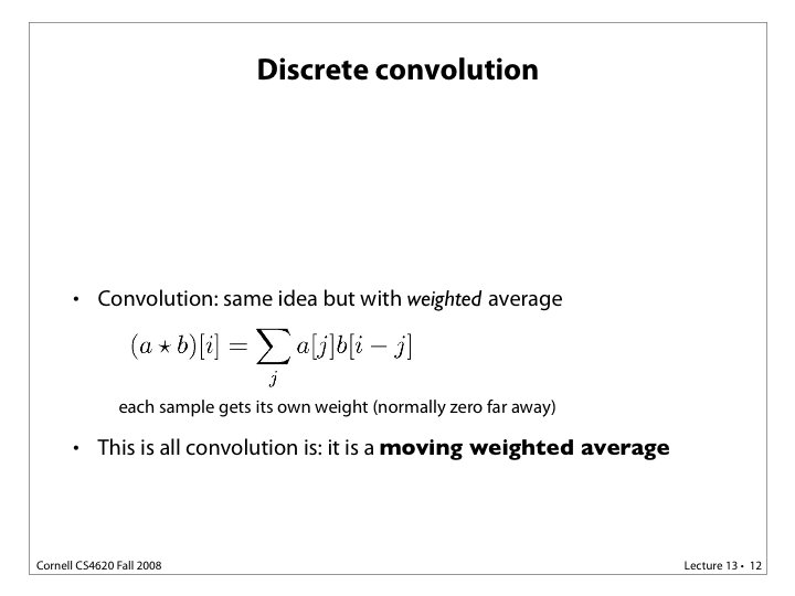
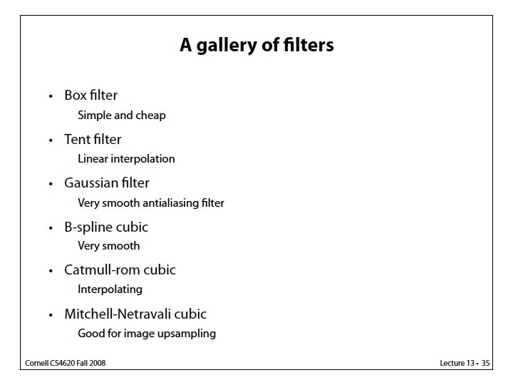
Reconstruction using 1 D tent filter 1 D example: g[n+1] g[n] n-1 n x n+1 n+2 Tent filter reconstruction: Zero-order continuity Use only one multiplication?

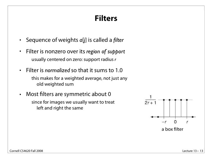
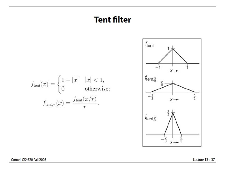
Infinitely smooth, negligible beyond [-3, 3]

C 2 Smoothness Can be obtained by convolving a box filter four times What’s the problem to use it as a reconstruction filter?

C 1 Smoothness It interpolates samples: “connecting the dots”

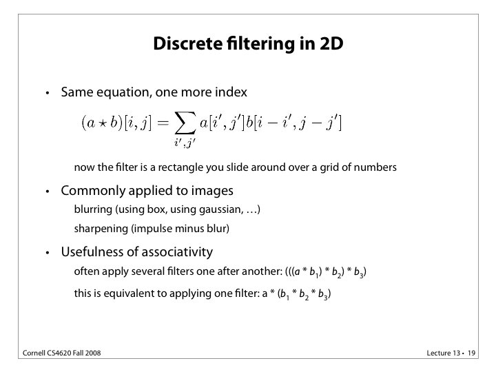
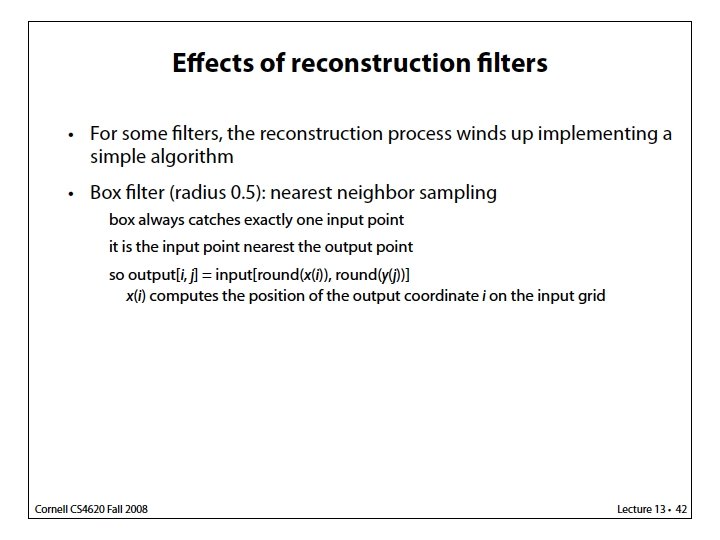
All-around best choice [Mitchell & Netravali 1988]

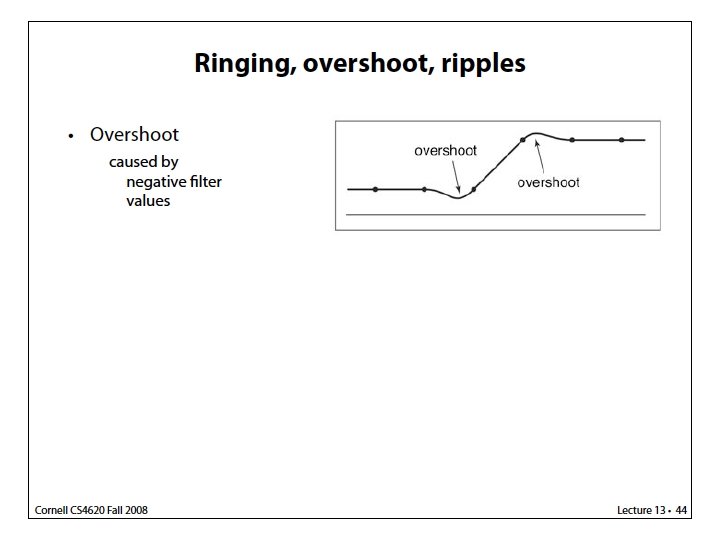
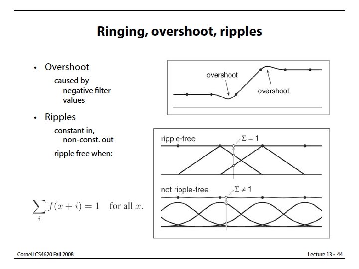
Properties of Kernels • Filter, Impulse Response, or kernel function, same concept but different names • Degrees of continuity • Interpolating or no • Ringing or overshooting Interpolating filter for reconstruction

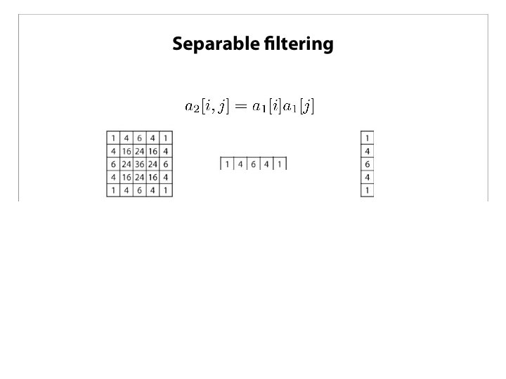
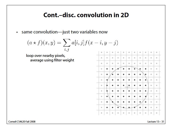
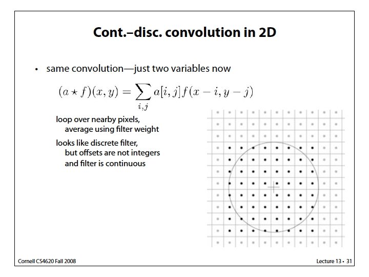
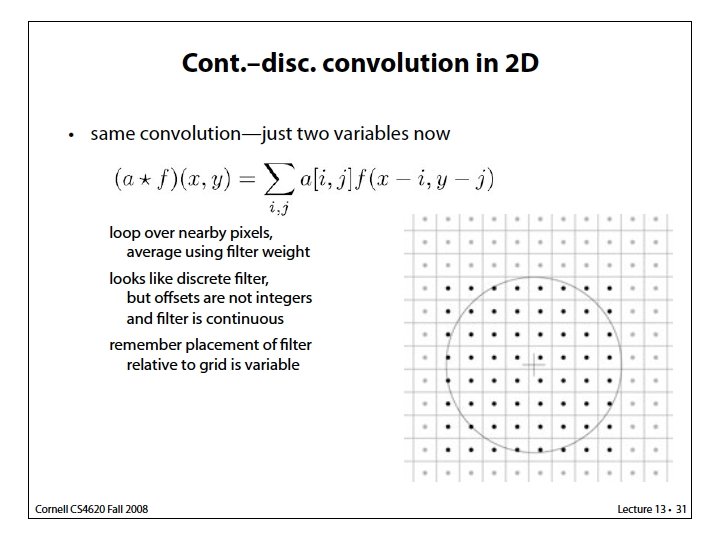
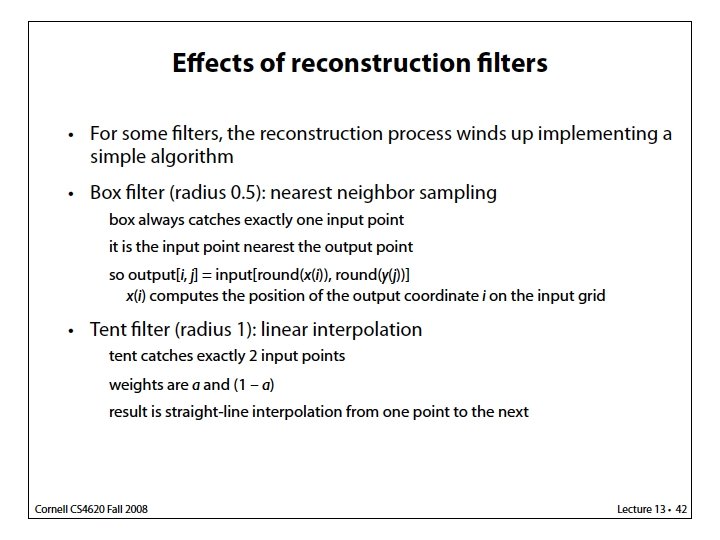
Reconstruction filter Examples in 2 D 2 D example: g[n+1, m] g[n, m] (x, y) g[n, m+1] g[n+1, m+1] How to simplify the calculation?

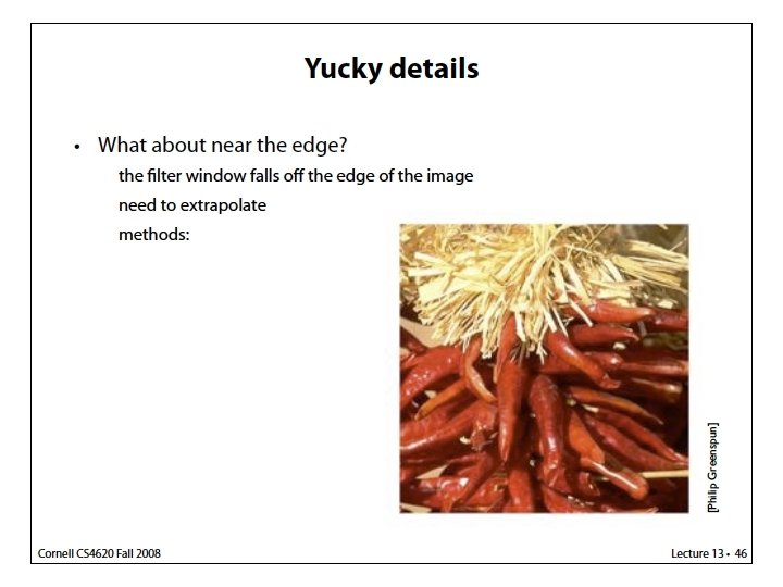
Image Filter Near Boundaries ? 0. 25 1 * 0. 5 3 9 4 5 0. 25 = • Kernel Renormalization 8 8 1 3 7

Image Filter Near Boundaries ? 0 1 * 0. 5 3 9 0. 25 / 0. 75 4 5 = • Kernel Renormalization 8 8 1 3 7

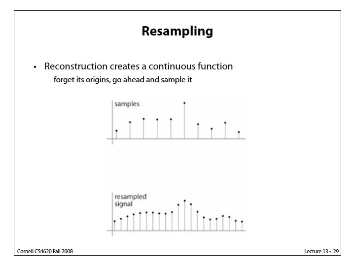
Practical upsampling • This can also be viewed as: 1. putting the reconstruction filter at the desired location 2. evaluating at the original sample positions 3. taking products with the sample values themselves 4. summing it up

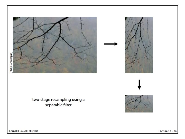
Image Downsampling 1/8 1/4 Throw away every other row and column to create a 1/2 size image - called image sub-sampling

Image sub-sampling 1/2 1/4 (2 x zoom) 1/8 (4 x zoom) Why does this look so crufty? Minimum Sampling requirement is not satisfied – resulting in Aliasing effect

Subsampling with Gaussian pre-filtering Gaussian 1/2 G 1/4 G 1/8 • Solution: filter the image, then subsample

Practical downsampling • Downsampling is similar, but filter has larger support and smaller amplitude. • Operationally: 1. Choose reconstruction filter in downsampled space. 2. Compute the downsampling rate, d, ratio of new sampling rate to old sampling rate 3. Stretch the filter by 1/d and scale it down by d 4. Follow upsampling procedure (previous slides) to compute new values (need normalization)

Filter Choice: speed vs quality Box filter: very fast Tent filter: moderate quality Cubic filter: excellent quality, for example Mitchell filter.