CS 559 Computer Graphics Lecture 7 Image Warping

CS 559: Computer Graphics Lecture 7: Image Warping and Morphing Li Zhang Spring 2010 Most slides borrowed from Yungyu Chuang

Last time: edge dection

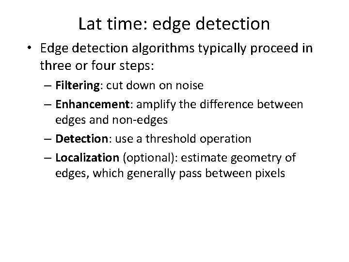
Lat time: edge detection • Edge detection algorithms typically proceed in three or four steps: – Filtering: cut down on noise – Enhancement: amplify the difference between edges and non-edges – Detection: use a threshold operation – Localization (optional): estimate geometry of edges, which generally pass between pixels

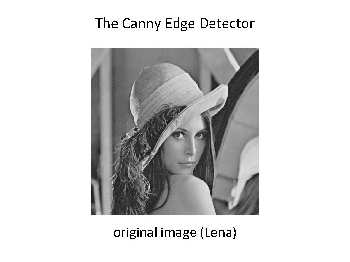
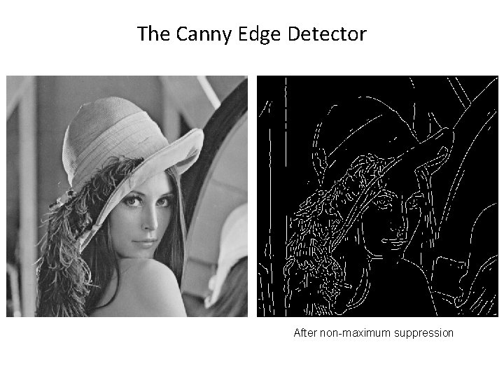
The Canny Edge Detector original image (Lena)

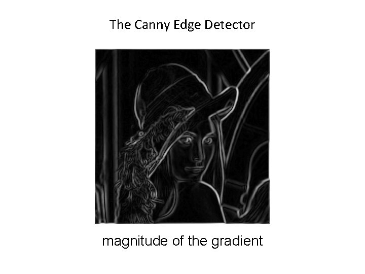
The Canny Edge Detector magnitude of the gradient

The Canny Edge Detector After non-maximum suppression

Lat time: edge detection • Edge detection algorithms typically proceed in three or four steps: – Filtering: cut down on noise – Enhancement: amplify the difference between edges and non-edges – Detection: use a threshold operation – Localization (optional): estimate geometry of edges, which generally pass between pixels

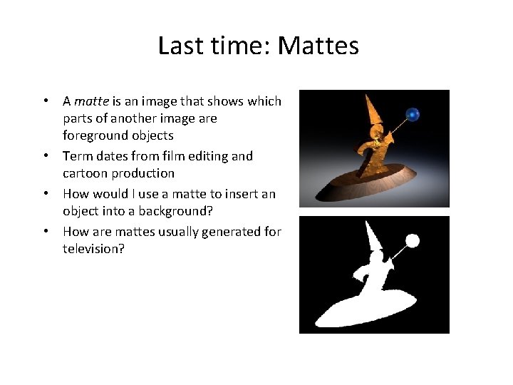
Last time: Mattes • A matte is an image that shows which parts of another image are foreground objects • Term dates from film editing and cartoon production • How would I use a matte to insert an object into a background? • How are mattes usually generated for television?

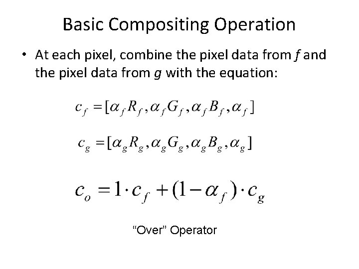
Basic Compositing Operation • At each pixel, combine the pixel data from f and the pixel data from g with the equation: “Over” Operator

Last time: 2 D Transformations h([x, y])=[x, y/2] T p = (x, y) p’ = (x’, y’) • Transformation T is a coordinate-changing machine: p’ = T(p) • What does it mean that T is global? – can be described by just a few numbers (parameters) – the parameters are the same for any point p • Represent T as a matrix: p’ = Mp

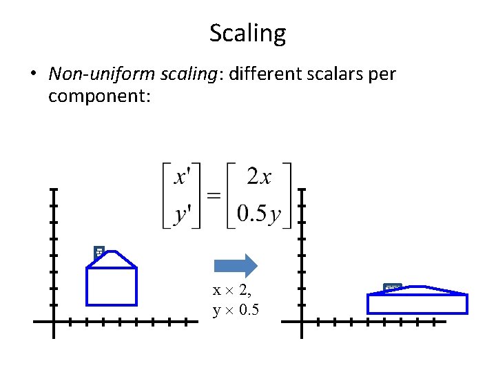
Scaling • Non-uniform scaling: different scalars per component: x 2, y 0. 5

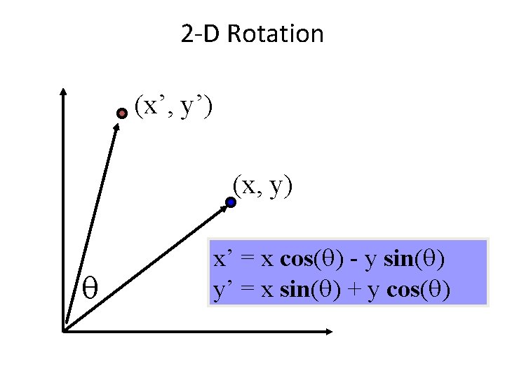
2 -D Rotation (x’, y’) (x, y) x’ = x cos( ) - y sin( ) y’ = x sin( ) + y cos( )

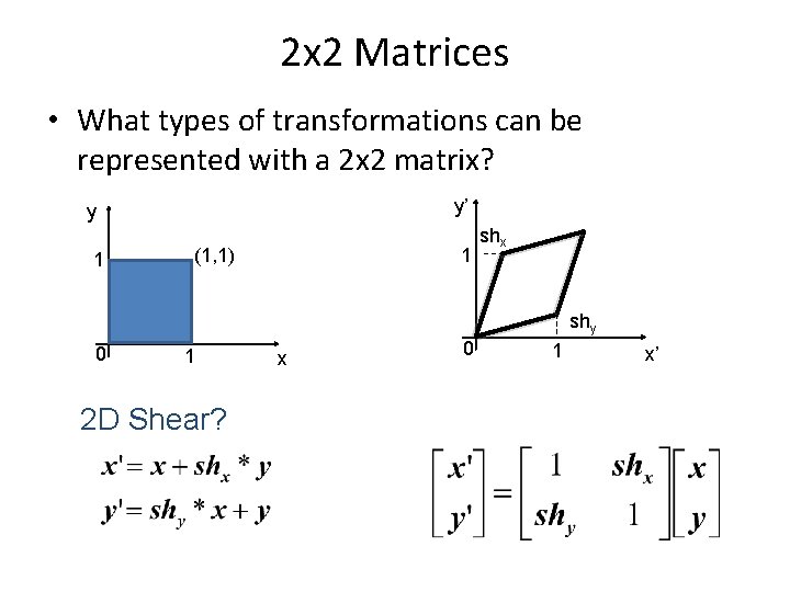
2 x 2 Matrices • What types of transformations can be represented with a 2 x 2 matrix? y’ y 1 1 (1, 1) shx shy 0 1 2 D Shear? x 0 1 x’

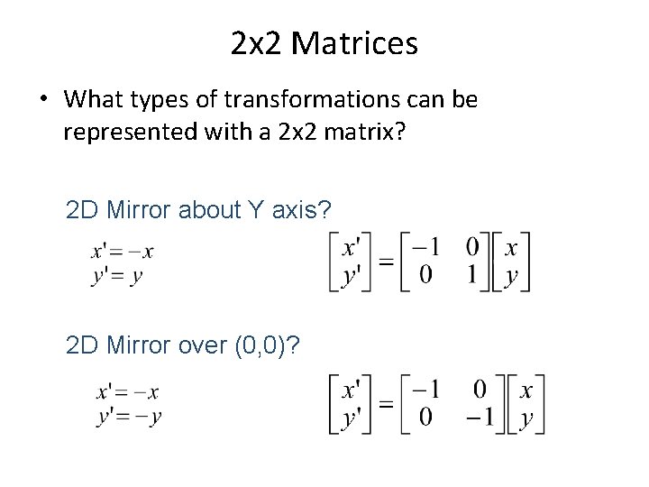
2 x 2 Matrices • What types of transformations can be represented with a 2 x 2 matrix? 2 D Mirror about Y axis? 2 D Mirror over (0, 0)?

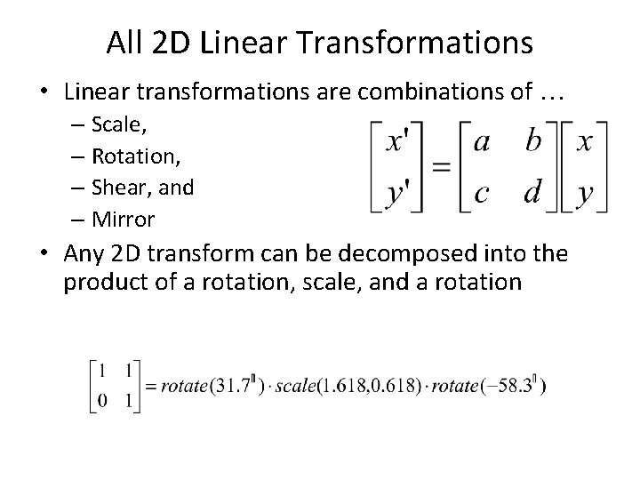
All 2 D Linear Transformations • Linear transformations are combinations of … – Scale, – Rotation, – Shear, and – Mirror • Any 2 D transform can be decomposed into the product of a rotation, scale, and a rotation

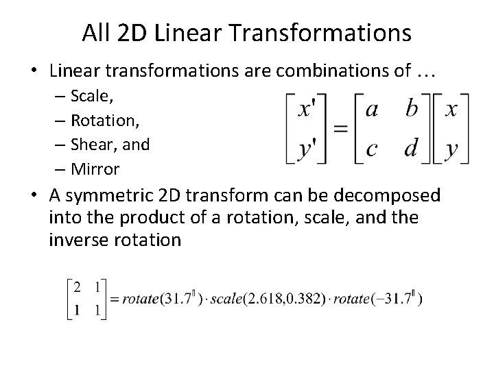
All 2 D Linear Transformations • Linear transformations are combinations of … – Scale, – Rotation, – Shear, and – Mirror • A symmetric 2 D transform can be decomposed into the product of a rotation, scale, and the inverse rotation

Today • More on 2 D transformation • Use it for image warping and morphing

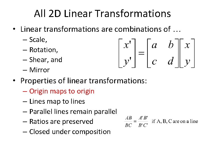
All 2 D Linear Transformations • Linear transformations are combinations of … – Scale, – Rotation, – Shear, and – Mirror • Properties of linear transformations: – Origin maps to origin – Lines map to lines – Parallel lines remain parallel – Ratios are preserved – Closed under composition

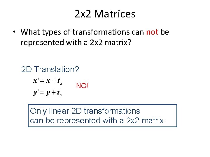
2 x 2 Matrices • What types of transformations can not be represented with a 2 x 2 matrix? 2 D Translation? NO! Only linear 2 D transformations can be represented with a 2 x 2 matrix

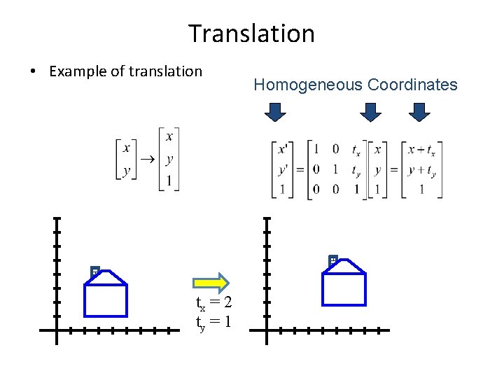
Translation • Example of translation tx = 2 ty = 1 Homogeneous Coordinates

Homogeneous coordinates • Why do we need it? – Can express all linear transformation as special cases

Homogeneous coordinates • Why do we need it? – Can express all linear transformation as special cases – Easy to compute a composite transformation that involve several translations and linear transformation

Homogeneous coordinates • Why do we need it? – Can express all linear transformation as special cases – Easy to compute a composite transformation that involve several translations and linear transformation – More to come

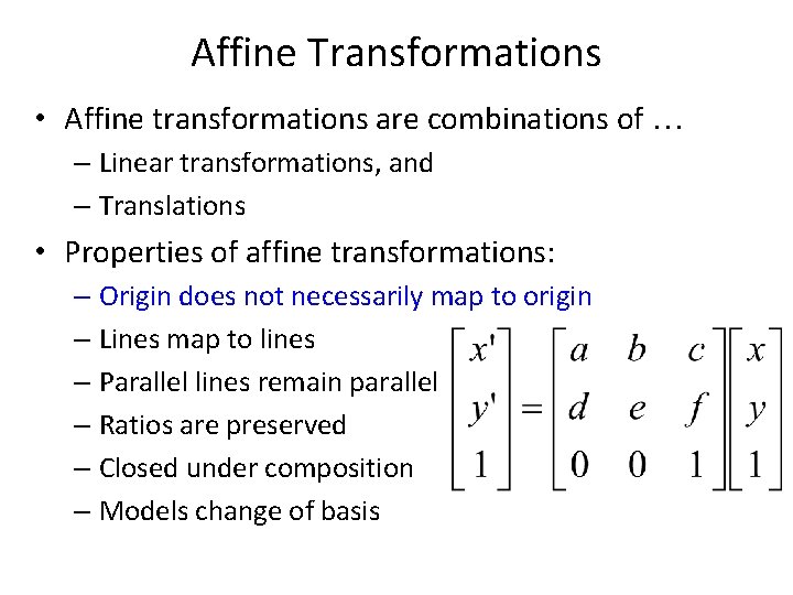
Affine Transformations • Affine transformations are combinations of … – Linear transformations, and – Translations • Properties of affine transformations: – Origin does not necessarily map to origin – Lines map to lines – Parallel lines remain parallel – Ratios are preserved – Closed under composition – Models change of basis

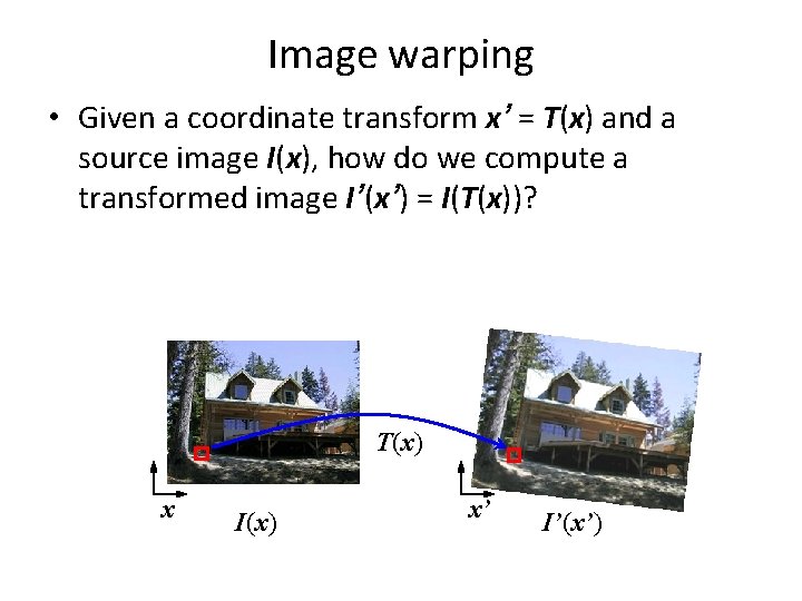
Image warping • Given a coordinate transform x’ = T(x) and a source image I(x), how do we compute a transformed image I’(x’) = I(T(x))? T(x) x I(x) x’ I’(x’)

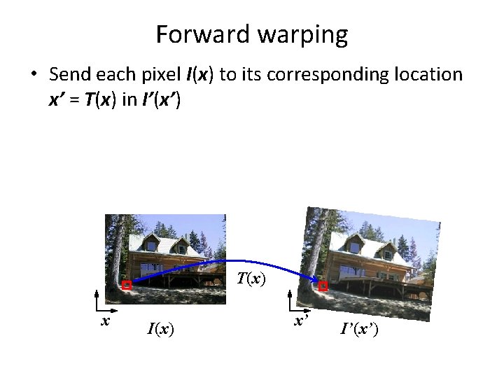
Forward warping • Send each pixel I(x) to its corresponding location x’ = T(x) in I’(x’) T(x) x I(x) x’ I’(x’)

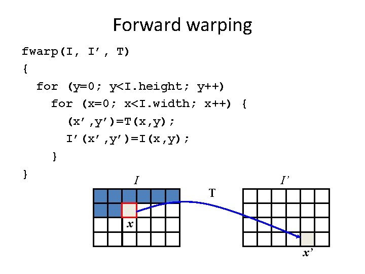
Forward warping fwarp(I, I’, T) { for (y=0; y<I. height; y++) for (x=0; x<I. width; x++) { (x’, y’)=T(x, y); I’(x’, y’)=I(x, y); } } I T I’ x x’

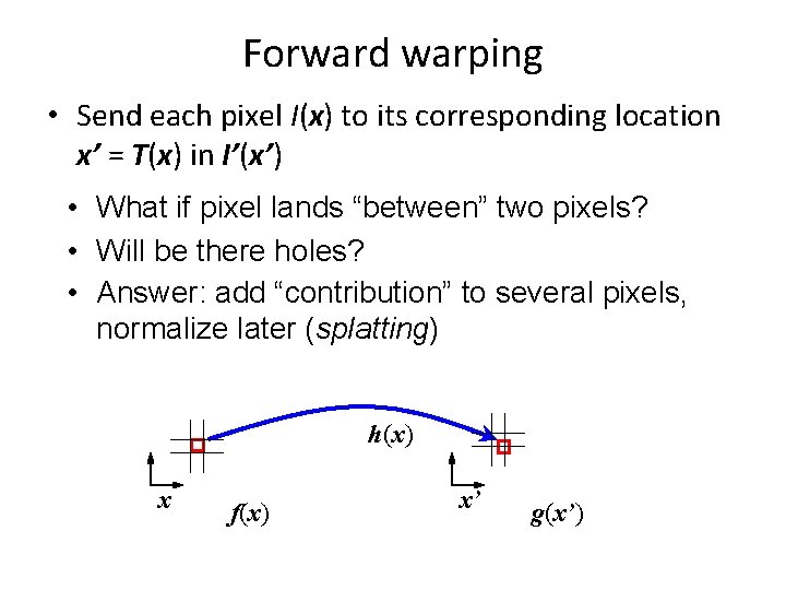
Forward warping • Send each pixel I(x) to its corresponding location x’ = T(x) in I’(x’) • What if pixel lands “between” two pixels? • Will be there holes? • Answer: add “contribution” to several pixels, normalize later (splatting) h(x) x f(x) x’ g(x’)

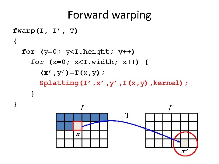
Forward warping fwarp(I, I’, T) { for (y=0; y<I. height; y++) for (x=0; x<I. width; x++) { (x’, y’)=T(x, y); Splatting(I’, x’, y’, I(x, y), kernel); } } I I’ T x x’

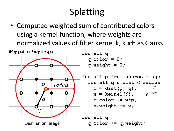
Splatting • Computed weighted sum of contributed colors using a kernel function, where weights are normalized values of filter kernel k, such as Gauss May get a blurry image! p radius d q Destination Image for all q q. color = 0; q. weight = 0; for all p from source image for all q’s dist < radius d = dist(p, q); w = kernel(d); q. color += w*p; q. weight += w; for all q q. Color /= q. weight;

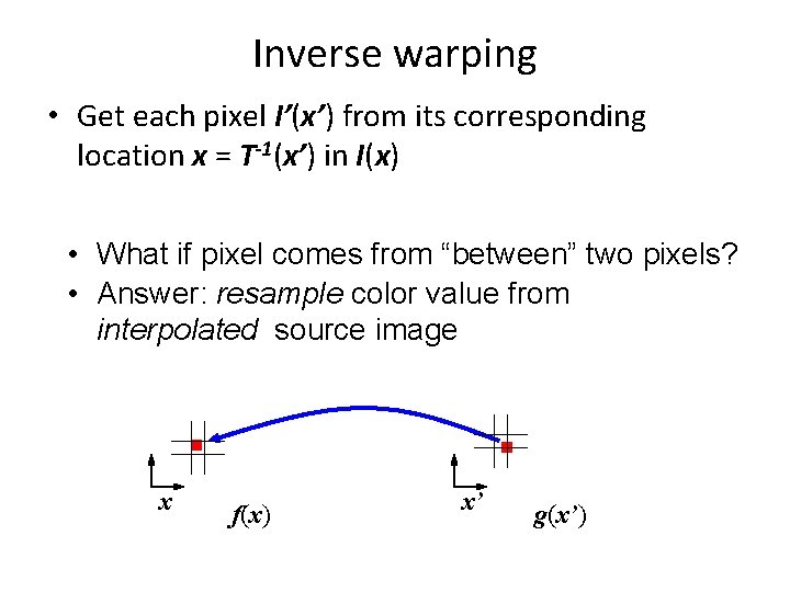
Inverse warping • Get each pixel I’(x’) from its corresponding location x = T-1(x’) in I(x) T-1(x’) x I(x) x’ I’(x’)

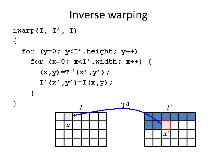
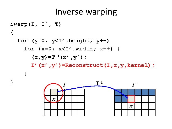
Inverse warping iwarp(I, I’, T) { for (y=0; y<I’. height; y++) for (x=0; x<I’. width; x++) { (x, y)=T-1(x’, y’); I’(x’, y’)=I(x, y); } } T-1 I I’ x x’

Inverse warping • Get each pixel I’(x’) from its corresponding location x = T-1(x’) in I(x) • What if pixel comes from “between” two pixels? • Answer: resample color value from interpolated source image x f(x) x’ g(x’)

Inverse warping iwarp(I, I’, T) { for (y=0; y<I’. height; y++) for (x=0; x<I’. width; x++) { (x, y)=T-1(x’, y’); I’(x’, y’)=Reconstruct(I, x, y, kernel); } } T-1 I I’ x x’

Reconstruction (interpolation) • Possible reconstruction filters (kernels): – nearest neighbor – bilinear – bicubic – sinc

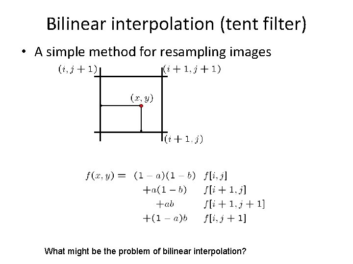
Bilinear interpolation (tent filter) • A simple method for resampling images What might be the problem of bilinear interpolation?

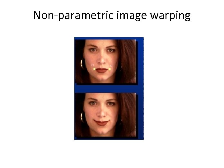
Non-parametric image warping

Non-parametric image warping • Specify a more detailed warp function [x, y] T [x’, y’]

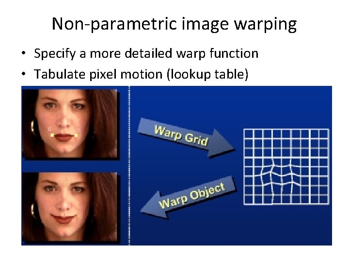
Non-parametric image warping • Specify a more detailed warp function • Tabulate pixel motion (lookup table)

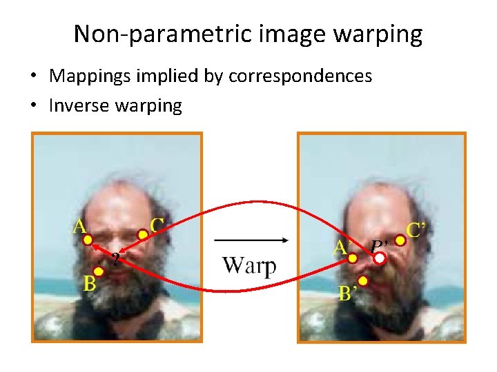
Non-parametric image warping • Mappings implied by correspondences • Inverse warping ? P’

Non-parametric image warping

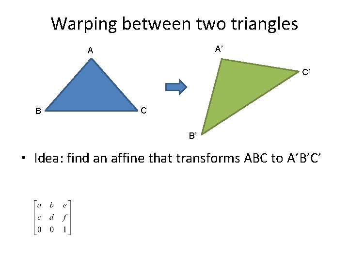
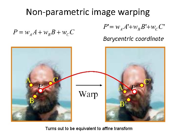
Warping between two triangles A’ A C’ B C B’ • Idea: find an affine that transforms ABC to A’B’C’

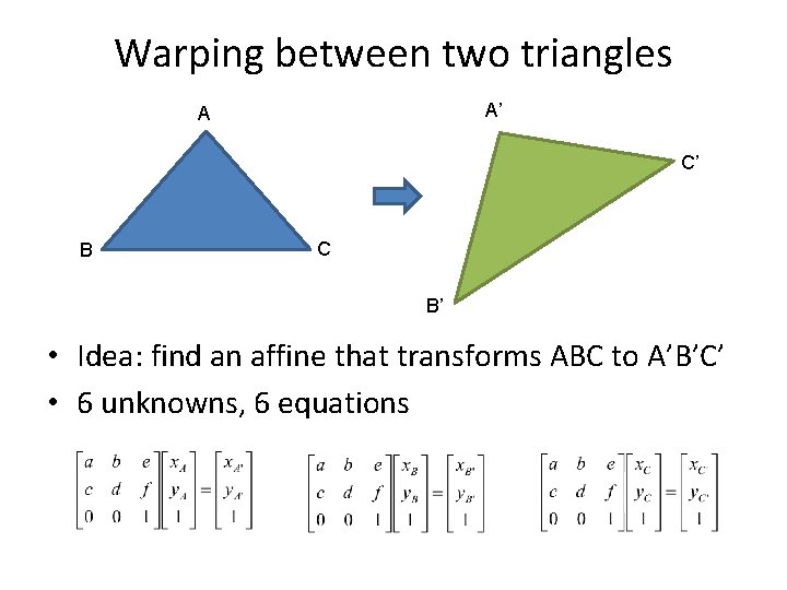
Warping between two triangles A’ A C’ B C B’ • Idea: find an affine that transforms ABC to A’B’C’ • 6 unknowns, 6 equations

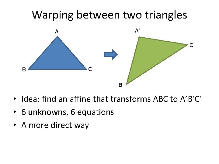
Warping between two triangles A’ A C’ B C B’ • Idea: find an affine that transforms ABC to A’B’C’ • 6 unknowns, 6 equations • A more direct way

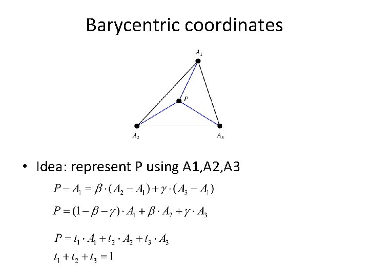
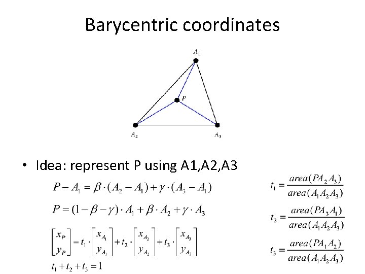
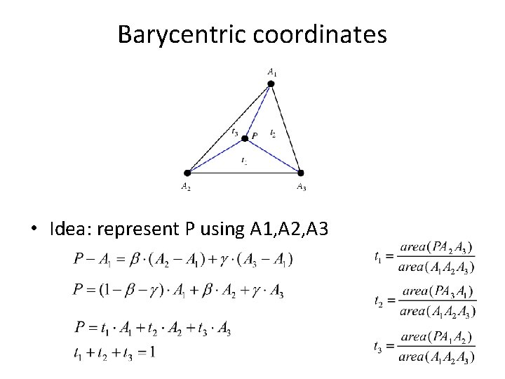
Barycentric coordinates • Idea: represent P using A 1, A 2, A 3

Barycentric coordinates • Idea: represent P using A 1, A 2, A 3

Barycentric coordinates • Idea: represent P using A 1, A 2, A 3

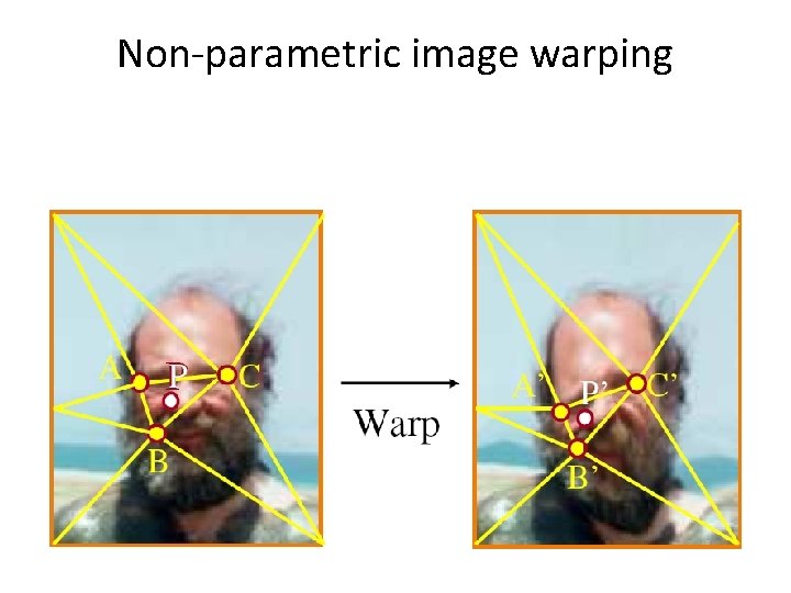
Non-parametric image warping Barycentric coordinate P P’ Turns out to be equivalent to affine transform