CS 3291 Sect 2 Review of analogue systems

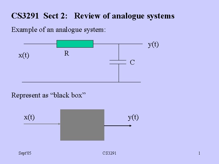
CS 3291 Sect 2: Review of analogue systems Example of an analogue system: y(t) x(t) R C Represent as “black box” x(t) Sept'05 y(t) CS 3291 1

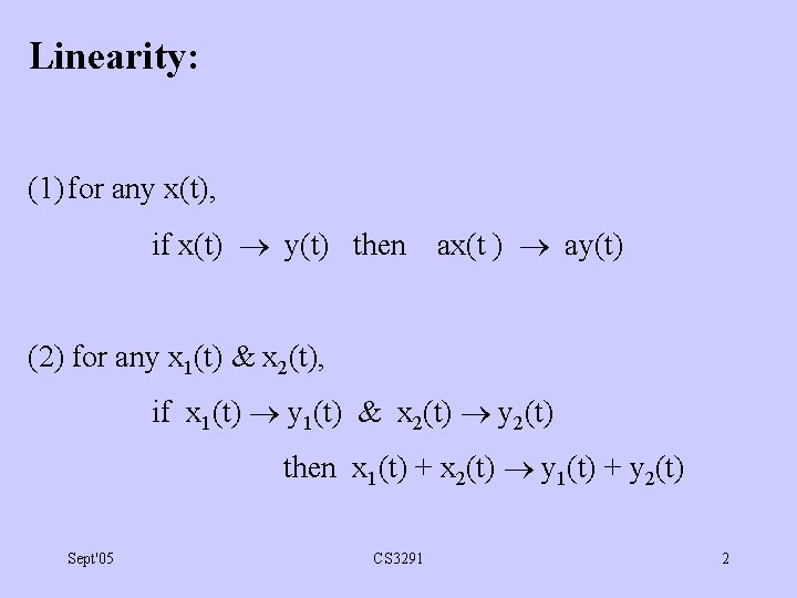
Linearity: (1) for any x(t), if x(t) y(t) then ax(t ) ay(t) (2) for any x 1(t) & x 2(t), if x 1(t) y 1(t) & x 2(t) y 2(t) then x 1(t) + x 2(t) y 1(t) + y 2(t) Sept'05 CS 3291 2

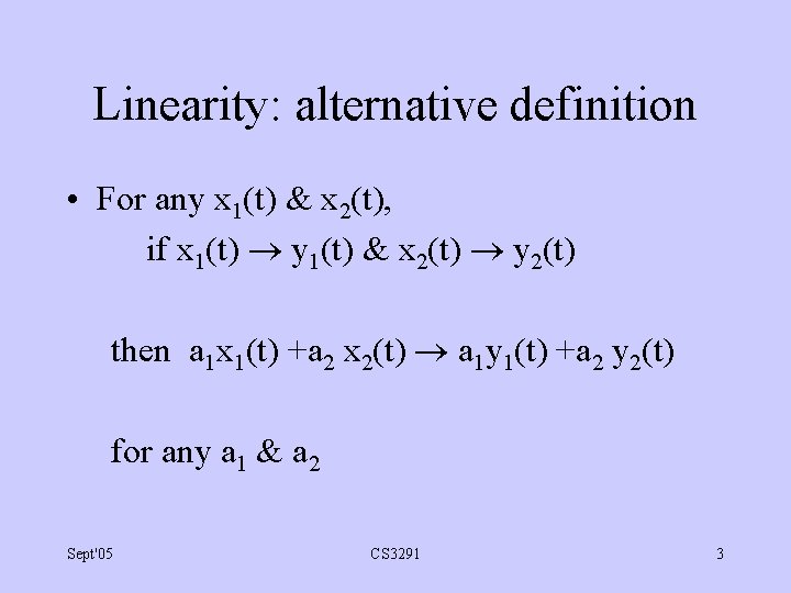
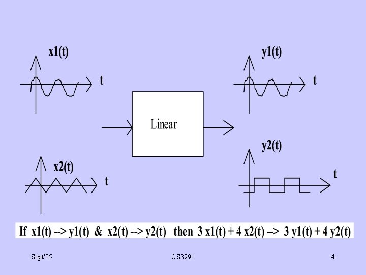
Linearity: alternative definition • For any x 1(t) & x 2(t), if x 1(t) y 1(t) & x 2(t) y 2(t) then a 1 x 1(t) +a 2 x 2(t) a 1 y 1(t) +a 2 y 2(t) for any a 1 & a 2 Sept'05 CS 3291 3

Sept'05 CS 3291 4

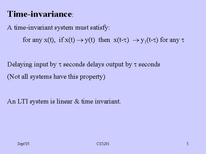
Time-invariance: A time-invariant system must satisfy: for any x(t), if x(t) y(t) then x(t- ) y 1(t- ) for any Delaying input by seconds delays output by seconds (Not all systems have this property) An LTI system is linear & time invariant. Sept'05 CS 3291 5

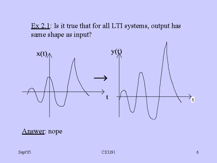
Ex 2. 1: Is it true that for all LTI systems, output has same shape as input? Answer: nope Sept'05 CS 3291 6

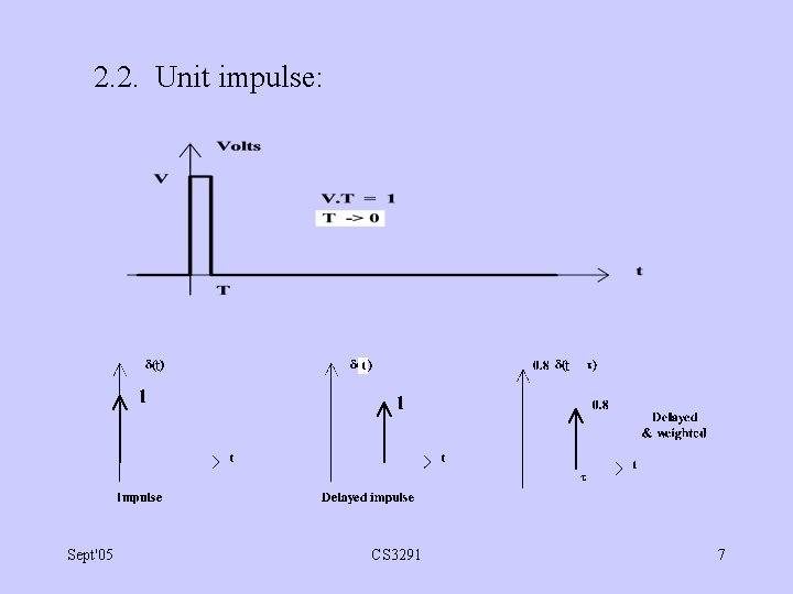
2. 2. Unit impulse: Sept'05 CS 3291 7

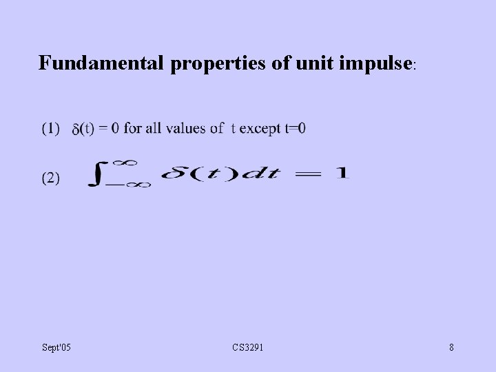
Fundamental properties of unit impulse: Sept'05 CS 3291 8

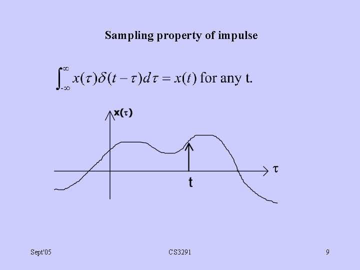
Sampling property of impulse Sept'05 CS 3291 9

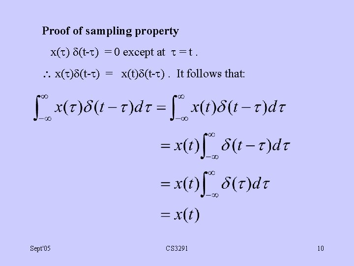
Proof of sampling property x( ) (t- ) = 0 except at = t. x( ) (t- ) = x(t) (t- ). It follows that: Sept'05 CS 3291 10

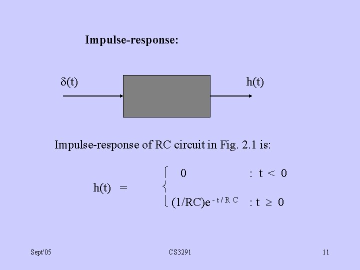
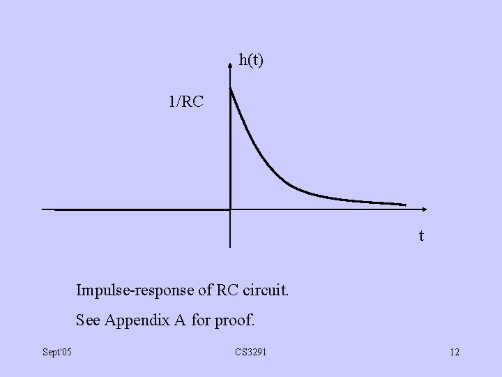
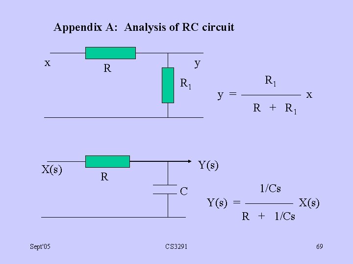
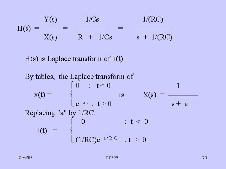
Impulse-response: (t) h(t) Impulse-response of RC circuit in Fig. 2. 1 is: h(t) = Sept'05 0 : t < 0 (1/RC)e - t / R C : t 0 CS 3291 11

h(t) 1/RC t Impulse-response of RC circuit. See Appendix A for proof. Sept'05 CS 3291 12

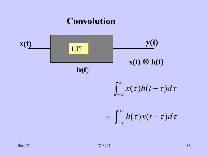
Convolution x(t) y(t) LTI x(t) h(t) Sept'05 CS 3291 13

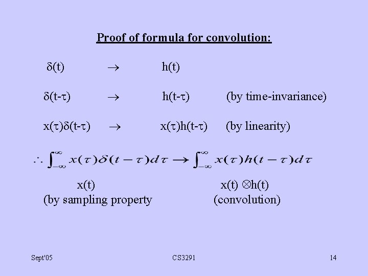
Proof of formula for convolution: (t) h(t) (t- ) h(t- ) (by time-invariance) x( ) (t- ) x( )h(t- ) (by linearity) x(t) h(t) (convolution) x(t) (by sampling property Sept'05 CS 3291 14

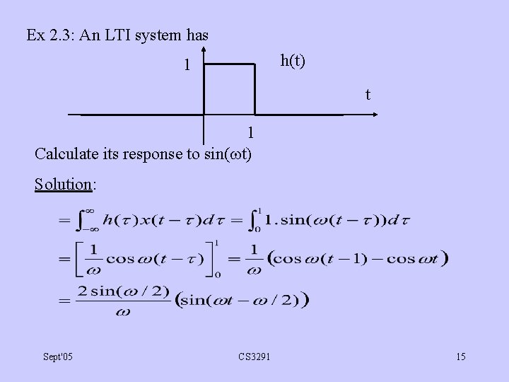
Ex 2. 3: An LTI system has h(t) 1 t 1 Calculate its response to sin( t) Solution: Sept'05 CS 3291 15

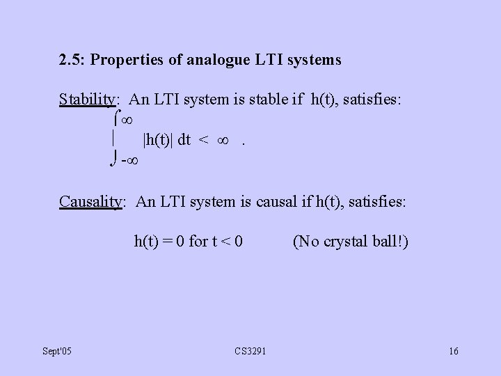
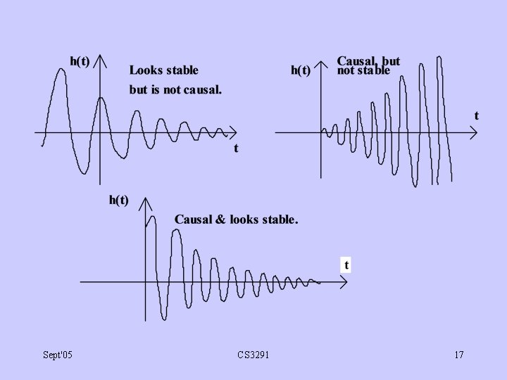
2. 5: Properties of analogue LTI systems Stability: An LTI system is stable if h(t), satisfies: |h(t)| dt < . - Causality: An LTI system is causal if h(t), satisfies: h(t) = 0 for t < 0 Sept'05 CS 3291 (No crystal ball!) 16

Sept'05 CS 3291 17

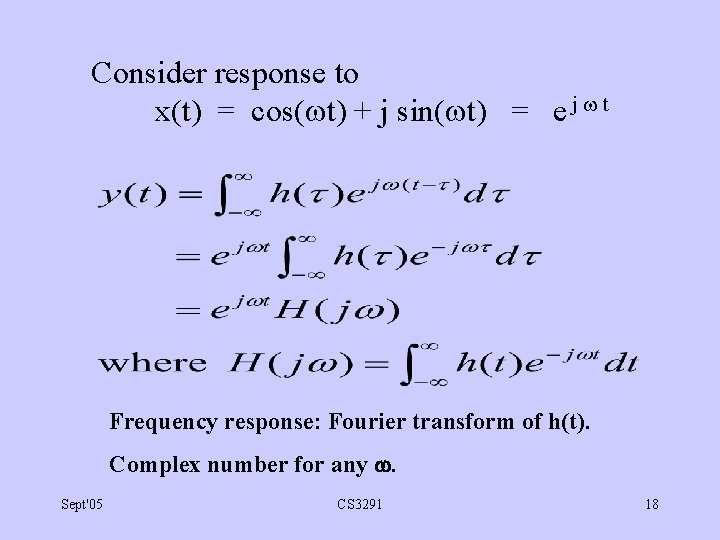
Consider response to x(t) = cos( t) + j sin( t) = e j t Frequency response: Fourier transform of h(t). Complex number for any . Sept'05 CS 3291 18

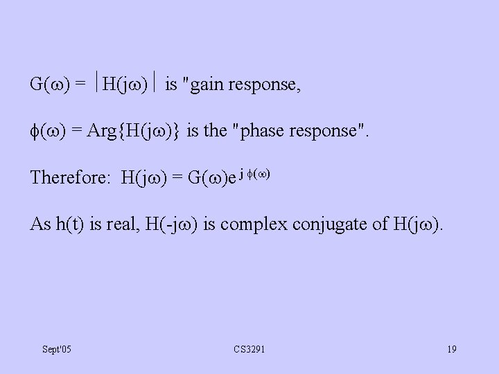
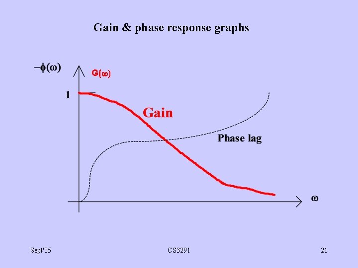
G( ) = H(j ) is "gain response, ( ) = Arg{H(j )} is the "phase response". Therefore: H(j ) = G( )e j ( ) As h(t) is real, H(-j ) is complex conjugate of H(j ). Sept'05 CS 3291 19

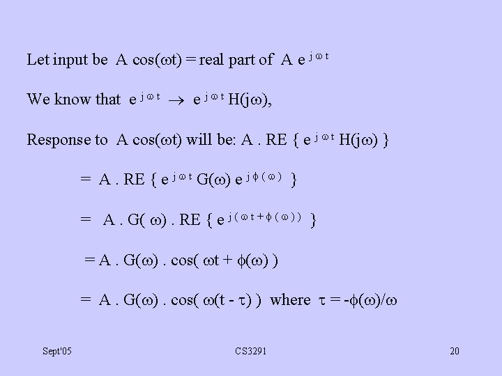
Let input be A cos( t) = real part of A e j t We know that e j t H(j ), Response to A cos( t) will be: A. RE { e j t H(j ) } = A. RE { e j t G( ) e j ( ) } = A. G( ). RE { e j ( t + ( ) ) } = A. G( ). cos( t + ( ) ) = A. G( ). cos( (t - ) ) where = - ( )/ Sept'05 CS 3291 20

Gain & phase response graphs G( ) Sept'05 CS 3291 21

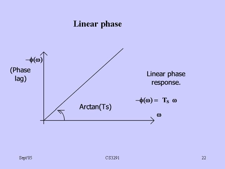
Linear phase Sept'05 CS 3291 22

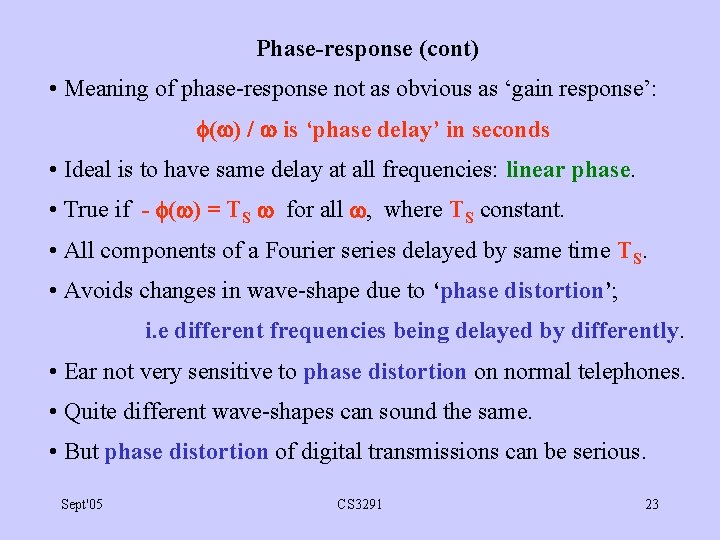
Phase-response (cont) • Meaning of phase-response not as obvious as ‘gain response’: ( ) / is ‘phase delay’ in seconds • Ideal is to have same delay at all frequencies: linear phase. • True if - ( ) = TS for all , where TS constant. • All components of a Fourier series delayed by same time TS. • Avoids changes in wave-shape due to ‘phase distortion’; i. e different frequencies being delayed by differently. • Ear not very sensitive to phase distortion on normal telephones. • Quite different wave-shapes can sound the same. • But phase distortion of digital transmissions can be serious. Sept'05 CS 3291 23

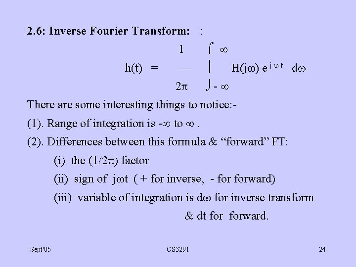
2. 6: Inverse Fourier Transform: : h(t) = 1 2 - H(j ) e j t d There are some interesting things to notice: (1). Range of integration is - to . (2). Differences between this formula & “forward” FT: (i) the (1/2 ) factor (ii) sign of j t ( + for inverse, - forward) (iii) variable of integration is d for inverse transform & dt forward. Sept'05 CS 3291 24

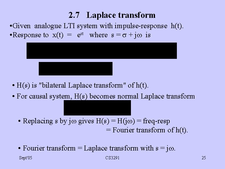
2. 7 Laplace transform • Given analogue LTI system with impulse-response h(t). • Response to x(t) = est where s = + j is • H(s) is "bilateral Laplace transform" of h(t). • For causal system, H(s) becomes normal Laplace transform • Replacing s by j gives H(s) = H(j ) = freq-resp = Fourier transform of h(t). • Fourier transform = Laplace transform with s = j. Sept'05 CS 3291 25

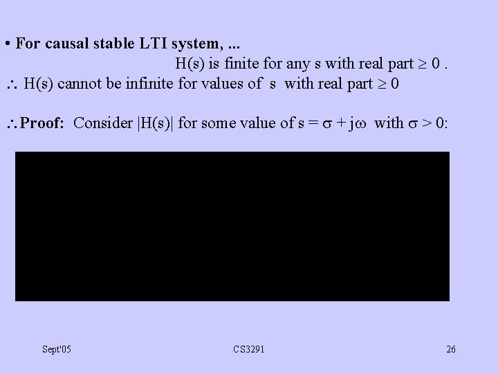
• For causal stable LTI system, . . . H(s) is finite for any s with real part 0. H(s) cannot be infinite for values of s with real part 0 Proof: Consider |H(s)| for some value of s = + j with > 0: Sept'05 CS 3291 26

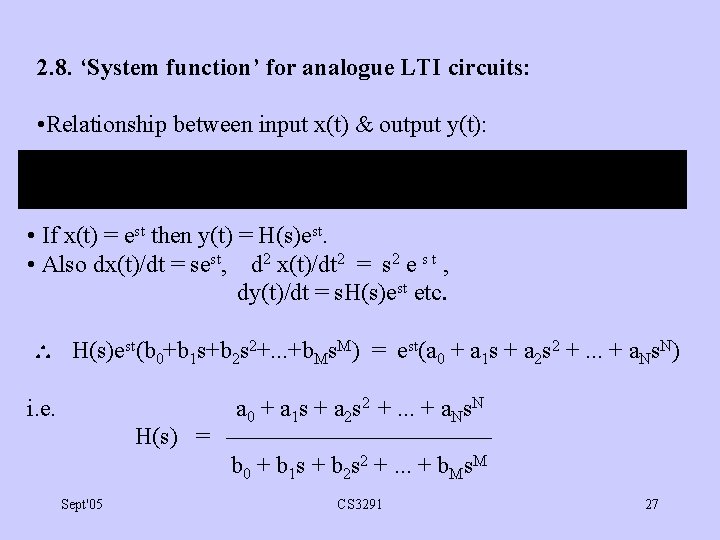
2. 8. ‘System function’ for analogue LTI circuits: • Relationship between input x(t) & output y(t): • If x(t) = est then y(t) = H(s)est. • Also dx(t)/dt = sest, d 2 x(t)/dt 2 = s 2 e s t , dy(t)/dt = s. H(s)est etc. H(s)est(b 0+b 1 s+b 2 s 2+. . . +b. Ms. M) = est(a 0 + a 1 s + a 2 s 2 +. . . + a. Ns. N) i. e. a 0 + a 1 s + a 2 s 2 +. . . + a. Ns. N H(s) = b 0 + b 1 s + b 2 s 2 +. . . + b. Ms. M Sept'05 CS 3291 27

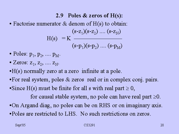
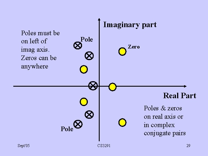
2. 9 Poles & zeros of H(s): • Factorise numerator & denom of H(s) to obtain: (s-z 1)(s-z 2). . (s-z. N) H(s) = K (s-p 1)(s-p 2). . (s-p. M) • Poles: p 1, p 2, . . p. M. • Zeros: z 1, z 2, . . z. N. • H(s) normally zero at a zero infinite at a pole. • For real system, poles & zeros real or in complex conj. pairs. • Since H(s) must be finite for all s with real part 0, for causal stable system, no pole can have real part 0. • On Argand diag, no poles can be on RHS or on imaginary axis. • Poles are restricted to LHS. No such restrictions on zeros. Sept'05 CS 3291 28

Imaginary part Poles must be on left of imag axis. Zeros can be anywhere Pole Zero Real Part Poles & zeros on real axis or in complex conjugate pairs Pole Sept'05 CS 3291 29

2. 10. Design of analogue filters • Two stages given a frequency response specification: 1) Find realisable H(s) which approximates the specification: 2) Find circuit to realise H(s): • Many design techniques for digital filters use the same approximations as are used for analogue filters. • It is useful to review one of these. Sept'05 CS 3291 30

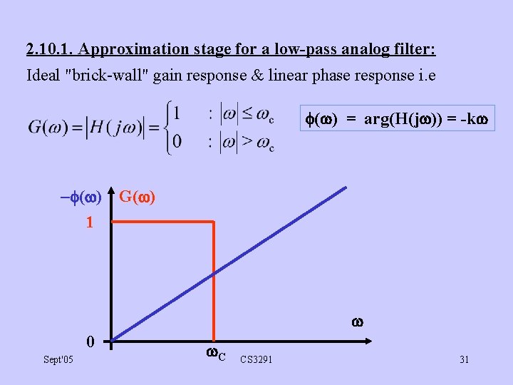
2. 10. 1. Approximation stage for a low-pass analog filter: Ideal "brick-wall" gain response & linear phase response i. e ( ) = arg(H(j )) = -k ( ) 1 G( ) 0 Sept'05 C CS 3291 31

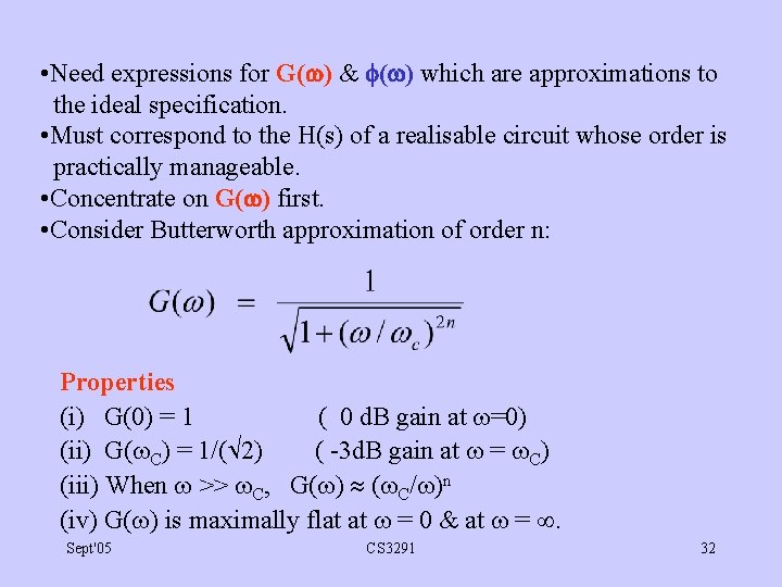
• Need expressions for G( ) & ( ) which are approximations to the ideal specification. • Must correspond to the H(s) of a realisable circuit whose order is practically manageable. • Concentrate on G( ) first. • Consider Butterworth approximation of order n: Properties (i) G(0) = 1 ( 0 d. B gain at =0) (ii) G( C) = 1/( 2) ( -3 d. B gain at = C) (iii) When >> C, G( ) ( C/ )n (iv) G( ) is maximally flat at = 0 & at = . Sept'05 CS 3291 32

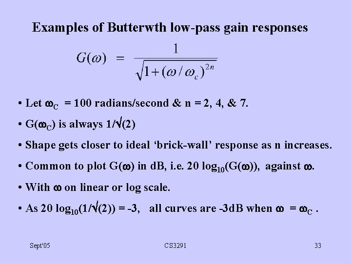
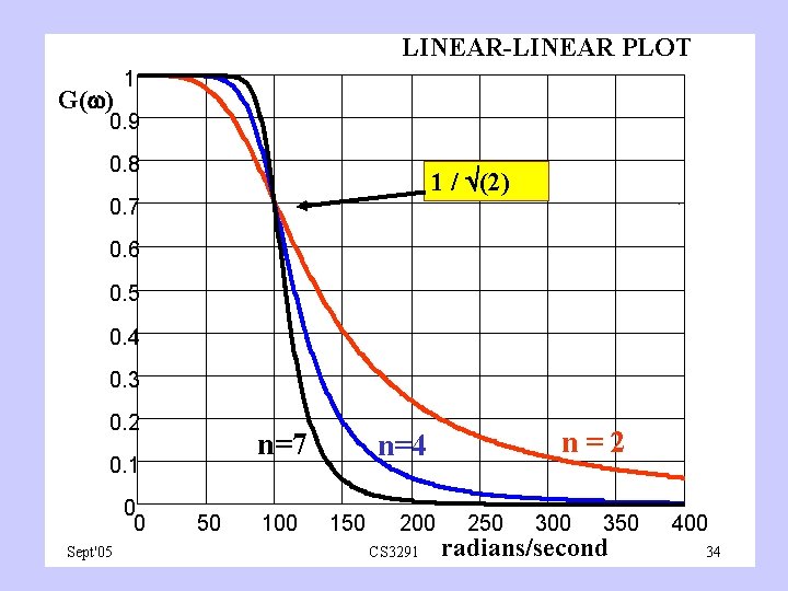
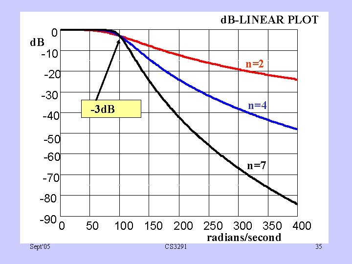
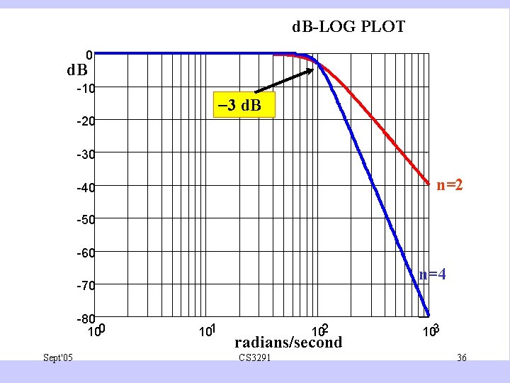
Examples of Butterwth low-pass gain responses • Let C = 100 radians/second & n = 2, 4, & 7. • G( C) is always 1/ (2) • Shape gets closer to ideal ‘brick-wall’ response as n increases. • Common to plot G( ) in d. B, i. e. 20 log 10(G( )), against . • With on linear or log scale. • As 20 log 10(1/ (2)) = -3, all curves are -3 d. B when = C. Sept'05 CS 3291 33

LINEAR-LINEAR PLOT G( ) 1 0. 9 0. 8 1 / (2) 0. 7 0. 6 0. 5 0. 4 0. 3 0. 2 n=7 0. 1 0 0 Sept'05 50 100 n=2 n=4 150 200 CS 3291 250 300 350 radians/second 400 34

d. B-LINEAR PLOT 0 d. B -10 n=2 -20 -30 -40 n=4 -3 d. B -50 -60 n=7 -70 -80 -90 Sept'05 0 50 100 150 200 250 300 350 400 radians/second CS 3291 35

d. B-LOG PLOT 0 d. B -10 3 d. B -20 -30 n=2 -40 -50 -60 n=4 -70 -80 100 Sept'05 101 102 radians/second CS 3291 103 36

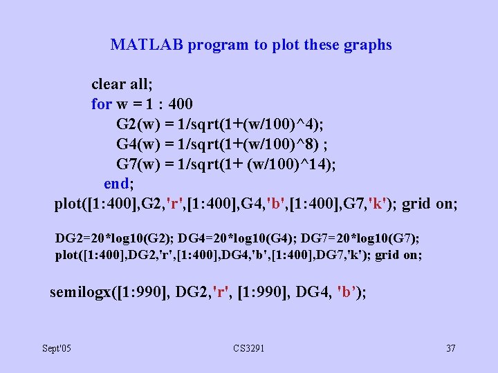
MATLAB program to plot these graphs clear all; for w = 1 : 400 G 2(w) = 1/sqrt(1+(w/100)^4); G 4(w) = 1/sqrt(1+(w/100)^8) ; G 7(w) = 1/sqrt(1+ (w/100)^14); end; plot([1: 400], G 2, 'r', [1: 400], G 4, 'b', [1: 400], G 7, 'k'); grid on; DG 2=20*log 10(G 2); DG 4=20*log 10(G 4); DG 7=20*log 10(G 7); plot([1: 400], DG 2, 'r', [1: 400], DG 4, 'b', [1: 400], DG 7, 'k'); grid on; semilogx([1: 990], DG 2, 'r', [1: 990], DG 4, 'b’); Sept'05 CS 3291 37

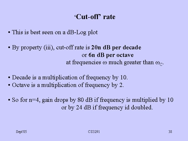
‘Cut-off’ rate • This is best seen on a d. B-Log plot • By property (iii), cut-off rate is 20 n d. B per decade or 6 n d. B per octave at frequencies much greater than C. • Decade is a multiplication of frequency by 10. • Octave is a multiplication of frequency by 2. • So for n=4, gain drops by 80 d. B if frequency is multiplied by 10 or by 24 d. B if frequency id doubled. Sept'05 CS 3291 38

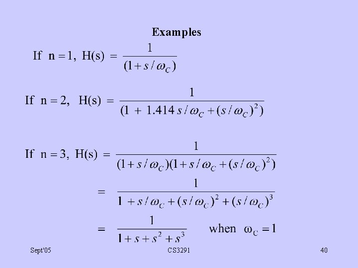
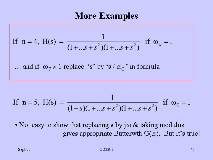
2. 10. 3 H(s) for nth order Butterworth low-pass approxn: H(s) = 1 [n/2] (1+s/ C)P {1 + 2 sin[(2 k-1) /2 n]s/ C + (s/ C)2} k=1 • [n/2] is integer part of n/2, • P=0 / 1 for n even/odd. sign means ‘product’. • Denominator is product of 1 st & 2 nd order polynomials in s. • H(s) is often realised by analogue circuits. • Can also be realised by IIR digital filters. Sept'05 CS 3291 39

Examples Sept'05 CS 3291 40

More Examples … and if C 1 replace ‘s’ by ‘s / C ’ in formula • Not easy to show that replacing s by j & taking modulus gives appropriate Butterwth G( ). But it’s true! Sept'05 CS 3291 41

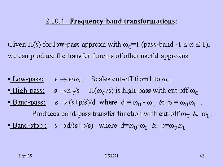
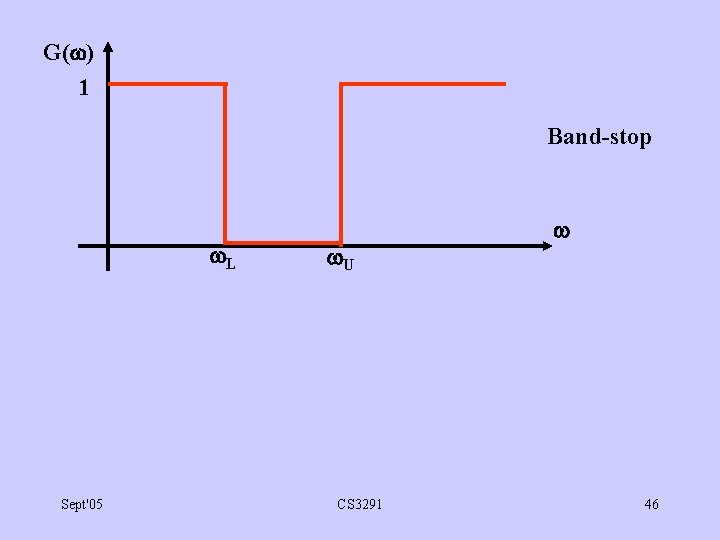
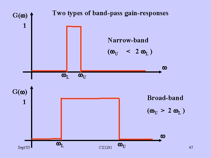
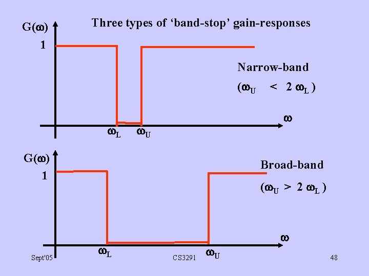
2. 10. 4 Frequency-band transformations: Given H(s) for low-pass approxn with C=1 (pass-band -1 1), we can produce the transfer functns of other useful approxns: • Low-pass: s s/ C Scales cut-off from 1 to C. • High-pass: s C/s • Band-pass: s (s+p/s)/d where d = U - L & p = U L. H( C /s) is high-pass with cut-off C Produces band-pass transfer function with cut-off U & L. • Band-stop : s d/(s+p/s) where d= U- L & p= U L Sept'05 CS 3291 42

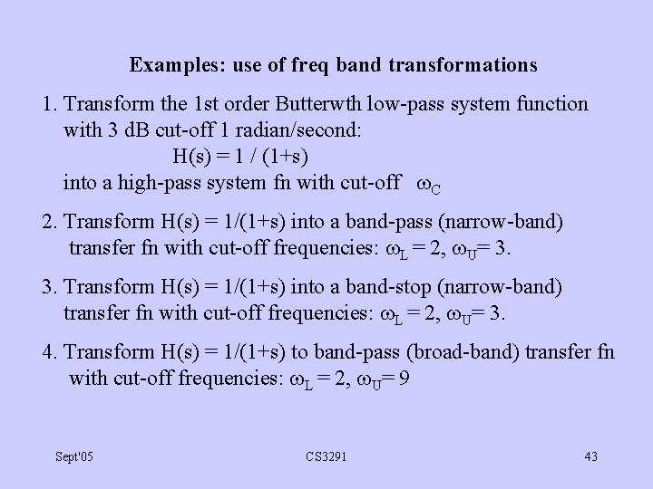
Examples: use of freq band transformations 1. Transform the 1 st order Butterwth low-pass system function with 3 d. B cut-off 1 radian/second: H(s) = 1 / (1+s) into a high-pass system fn with cut-off C 2. Transform H(s) = 1/(1+s) into a band-pass (narrow-band) transfer fn with cut-off frequencies: L = 2, U= 3. 3. Transform H(s) = 1/(1+s) into a band-stop (narrow-band) transfer fn with cut-off frequencies: L = 2, U= 3. 4. Transform H(s) = 1/(1+s) to band-pass (broad-band) transfer fn with cut-off frequencies: L = 2, U= 9 Sept'05 CS 3291 43

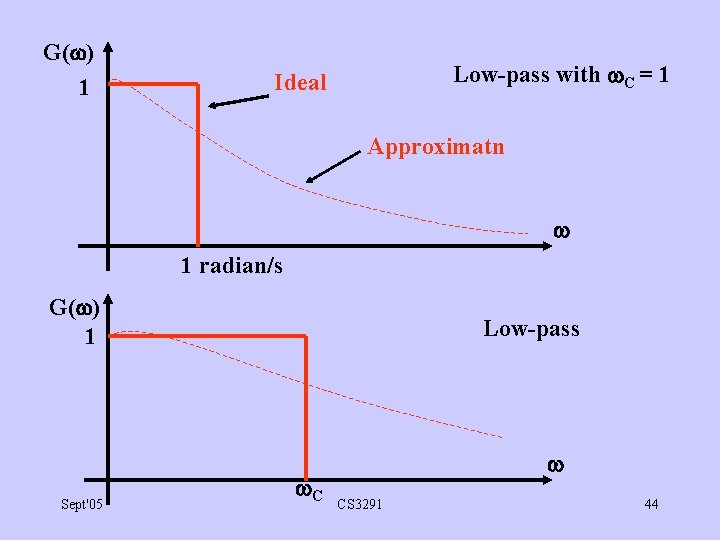
G( ) 1 Low-pass with C = 1 Ideal Approximatn 1 radian/s G( ) 1 Sept'05 Low-pass C CS 3291 44

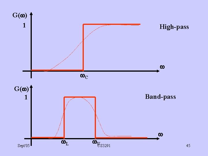
G( ) 1 High-pass C G( ) 1 Sept'05 Band-pass L U CS 3291 45

G( ) 1 Band-stop L Sept'05 U CS 3291 46

G( ) 1 Two types of band-pass gain-responses Narrow-band ( U L U G( ) 1 Sept'05 < 2 L ) Broad-band ( U > 2 L ) L CS 3291 U 47

G( ) 1 Three types of ‘band-stop’ gain-responses Narrow-band ( U L U G( ) 1 Sept'05 < 2 L ) Broad-band ( U > 2 L ) L CS 3291 U 48

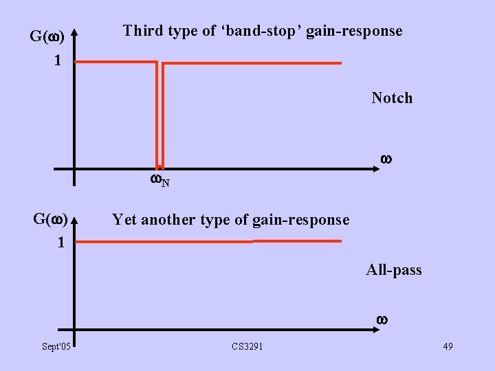
G( ) 1 Third type of ‘band-stop’ gain-response Notch N G( ) 1 Yet another type of gain-response All-pass Sept'05 CS 3291 49

Comments: • Given H(s) for low-pass gain-resp. with C =1, freq-band transfns always work & must be used for narrow-band. • ‘Broad-band’ band-pass & band-stop transfer fns can be obtained by combining low-pass & high-pass. • ‘Notch’ gain-resp. is band-stop with very narrow stop-band. Used for ‘notching out’ sinusoidal tone at one frequency. • All-pass gain-responses do nothing to magnitudes of sinusoids but can change their phases in useful ways. Sept'05 CS 3291 50

2. 11. Use of MATLAB for analogue filter design • High level language for matrix operations & complex numbers. • Ideal for studying & implementing signal processing operations. • Variables declared automatically when first used. • Each variable may be a matrix with complex elements. E. g. : X = [ 1 2 3 4 -5+3 j ]; % Comment • If semicolon omitted, print result of assignment. • It is easy to generate sections of sine-waves. • You need to know the sampling frequency f. S in Hz. • Can make f. S = 1 Hz which means 1 sample every second). Sept'05 CS 3291 51

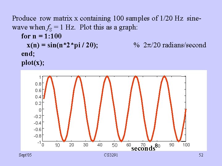
Produce row matrix x containing 100 samples of 1/20 Hz sinewave when f. S = 1 Hz. Plot this as a graph: for n = 1: 100 x(n) = sin(n*2*pi / 20); % 2 /20 radians/second end; plot(x); 1 0. 8 0. 6 0. 4 0. 2 0 -0. 2 -0. 4 -0. 6 -0. 8 -1 Sept'05 0 10 20 30 40 50 CS 3291 60 70 80 seconds 90 100 52

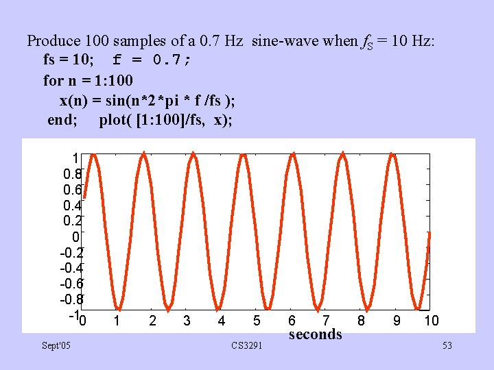
Produce 100 samples of a 0. 7 Hz sine-wave when f. S = 10 Hz: fs = 10; f = 0. 7; for n = 1: 100 x(n) = sin(n*2*pi * f /fs ); end; plot( [1: 100]/fs, x); 1 0. 8 0. 6 0. 4 0. 2 0 -0. 2 -0. 4 -0. 6 -0. 8 -10 Sept'05 1 2 3 4 5 CS 3291 6 7 seconds 8 9 10 53

• Note: ‘ [1: 100] / fs ’ is a row matrix [1, 2, …, 100] with each element divided by fs. • Following example shows how a WAV file containing speech or music may be read in, listened to & plotted in sections. • Sections may be processed and written to a second file. • ‘Control-C’ will interrupt a running MATLAB program even when in a infinite loop. Sept'05 CS 3291 54

clear all; [x, fs, nbits] = wavread('cap 4 th. wav'); SOUND(x, fs, nbits); for n=1: 1000 y(n)=x(n+10000); end; plot([1: 1000]/fs, y); wavwrite(y, fs, nbits, ’newfile. wav’); 0. 3 0. 2 0. 1 0 -0. 1 -0. 2 -0. 3 -0. 40 Sept'05 0. 015 0. 025 0. 035 0. 045 0. 05 CS 3291 55

2. 11. 1 MATLAB Signal Processing toolbox: A set of functions available to user of MATLAB for: (i) carrying out operations on signal segments stored in row matrices (ii) evaluating the effect of these operations, (iii) designing analogue & digital filters. Some of these functions are as follows: are: Sept'05 CS 3291 56

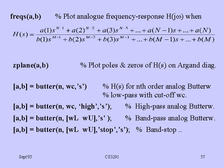
freqs(a, b) zplane(a, b) % Plot analogue frequency-response H(j ) when % Plot poles & zeros of H(s) on Argand diag. [a, b] = butter(n, wc, ’s’) % H(s) for nth order analog Butterw % low-pass with cut-off wc. [a, b] = butter(n, wc, ‘high’, ’s’); % High-pass analog Butterw. [a, b] = butter(n, [w. L w. U], ’s’ ); % Band-pass analog Butterw. [a, b] = butter(n, [w. L w. U], ’stop’, ’s’); % Band-stop. . Sept'05 CS 3291 57

Other analogue gain response approximations: [a, b] = cheby 1(n, Rp, wc, ’s’ ); % Low-pass Chebychev type 1. % Rp = pass-band ripple in d. B . [a, b] = cheby 2(n, Rs, wc, ’s’ ); (Slight error in notes (‘discrete time’) Sept'05 % Low-pass Chebychev type 2. % Rs = stop-band ripple in d. B . CS 3291 58

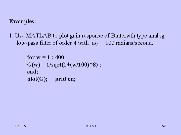
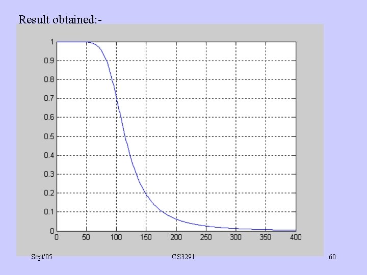
Examples: 1. Use MATLAB to plot gain response of Butterwth type analog low-pass filter of order 4 with C = 100 radians/second. for w = 1 : 400 G(w) = 1/sqrt(1+(w/100)^8) ; end; plot(G); grid on; Sept'05 CS 3291 59

Result obtained: - Sept'05 CS 3291 60

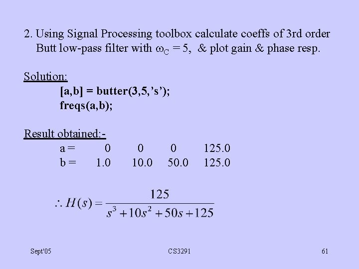
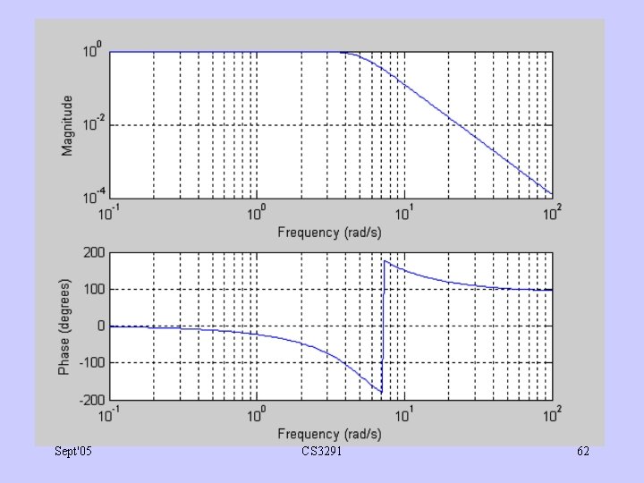
2. Using Signal Processing toolbox calculate coeffs of 3 rd order Butt low-pass filter with C = 5, & plot gain & phase resp. Solution: [a, b] = butter(3, 5, ’s’); freqs(a, b); Result obtained: a= 0 b= 1. 0 Sept'05 0 10. 0 0 50. 0 CS 3291 125. 0 61

Sept'05 CS 3291 62

Postscript • MATLAB goes not give H(s) with its denominator expressed in 2 nd order sections as our earlier formula did. • This is sometimes inconvenient. • As an exercise, find out how to use MATLAB to produce H(s) in 2 nd order sections. Sept'05 CS 3291 63

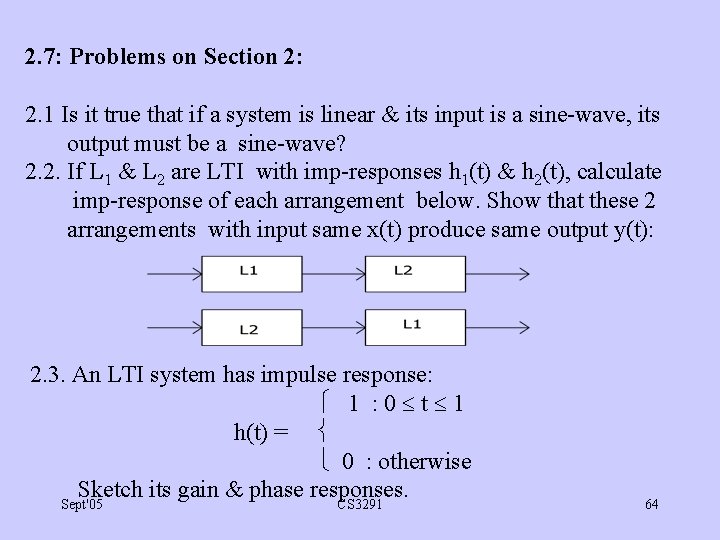
2. 7: Problems on Section 2: 2. 1 Is it true that if a system is linear & its input is a sine-wave, its output must be a sine-wave? 2. 2. If L 1 & L 2 are LTI with imp-responses h 1(t) & h 2(t), calculate imp-response of each arrangement below. Show that these 2 arrangements with input same x(t) produce same output y(t): 2. 3. An LTI system has impulse response: 1 : 0 t 1 h(t) = 0 : otherwise Sketch its gain & phase responses. Sept'05 CS 3291 64

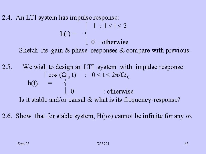
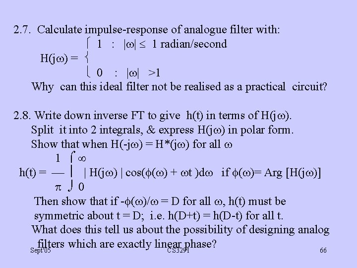
2. 4. An LTI system has impulse response: 1 : 1 t 2 h(t) = 0 : otherwise Sketch its gain & phase responses & compare with previous. 2. 5. We wish to design an LTI system with impulse response: cos ( 0 t) : 0 t 2 / 0 h(t) = 0 : otherwise Is it stable and/or causal & what is its frequency-response? 2. 6. Show that for stable system, H(j ) cannot be infinite for any . Sept'05 CS 3291 65

2. 7. Calculate impulse-response of analogue filter with: 1 : | | 1 radian/second H(j ) = 0 : | | >1 Why can this ideal filter not be realised as a practical circuit? 2. 8. Write down inverse FT to give h(t) in terms of H(j ). Split it into 2 integrals, & express H(j ) in polar form. Show that when H(-j ) = H*(j ) for all 1 h(t) = | H(j ) | cos( ( ) + t )d if ( )= Arg [H(j )] 0 Then show that if - ( )/ = D for all , h(t) must be symmetric about t = D; i. e. h(D+t) = h(D-t) for all t. What does this tell us about the possibility of designing analog filters which are exactly linear phase? Sept'05 CS 3291 66

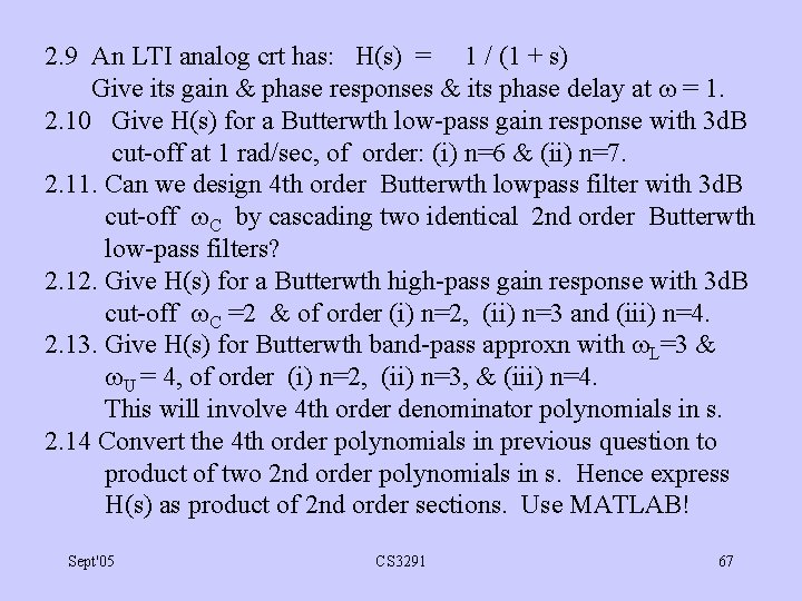
2. 9 An LTI analog crt has: H(s) = 1 / (1 + s) Give its gain & phase responses & its phase delay at = 1. 2. 10 Give H(s) for a Butterwth low-pass gain response with 3 d. B cut-off at 1 rad/sec, of order: (i) n=6 & (ii) n=7. 2. 11. Can we design 4 th order Butterwth lowpass filter with 3 d. B cut-off C by cascading two identical 2 nd order Butterwth low-pass filters? 2. 12. Give H(s) for a Butterwth high-pass gain response with 3 d. B cut-off C =2 & of order (i) n=2, (ii) n=3 and (iii) n=4. 2. 13. Give H(s) for Butterwth band-pass approxn with L=3 & U = 4, of order (i) n=2, (ii) n=3, & (iii) n=4. This will involve 4 th order denominator polynomials in s. 2. 14 Convert the 4 th order polynomials in previous question to product of two 2 nd order polynomials in s. Hence express H(s) as product of 2 nd order sections. Use MATLAB! Sept'05 CS 3291 67

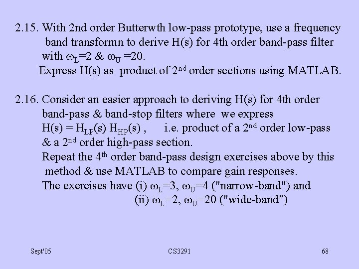
2. 15. With 2 nd order Butterwth low-pass prototype, use a frequency band transformn to derive H(s) for 4 th order band-pass filter with L=2 & U =20. Express H(s) as product of 2 nd order sections using MATLAB. 2. 16. Consider an easier approach to deriving H(s) for 4 th order band-pass & band-stop filters where we express H(s) = HLP(s) HHP(s) , i. e. product of a 2 nd order low-pass & a 2 nd order high-pass section. Repeat the 4 th order band-pass design exercises above by this method & use MATLAB to compare gain responses. The exercises have (i) L=3, U=4 ("narrow-band") and (ii) L=2, U=20 ("wide-band") Sept'05 CS 3291 68

Appendix A: Analysis of RC circuit x y R R 1 X(s) Y(s) R C Sept'05 R 1 y = x R + R 1 CS 3291 1/Cs Y(s) = X(s) R + 1/Cs 69

Y(s) H(s) = = X(s) 1/Cs = R + 1/Cs 1/(RC) s + 1/(RC) H(s) is Laplace transform of h(t). By tables, the Laplace transform of 0 : t<0 1 x(t) = is X(s) = e-at : t 0 s+ a Replacing "a" by 1/RC: 0 : t < 0 h(t) = (1/RC)e - t / R C : t 0 Sept'05 CS 3291 70