CMSC 635 Sampling and Antialiasing Aliasing in images

CMSC 635 Sampling and Antialiasing

Aliasing in images

Aliasing in animation

Aliasing § High frequencies alias as low frequencies

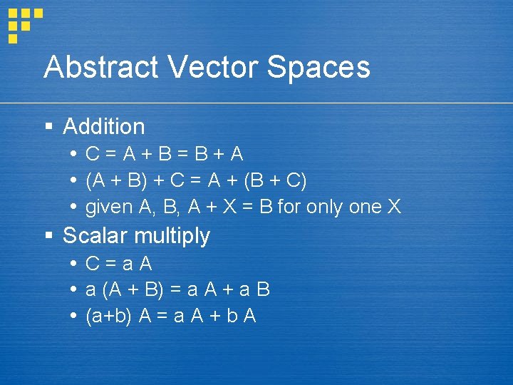
Abstract Vector Spaces § Addition C=A+B=B+A (A + B) + C = A + (B + C) given A, B, A + X = B for only one X § Scalar multiply C=a. A a (A + B) = a A + a B (a+b) A = a A + b A

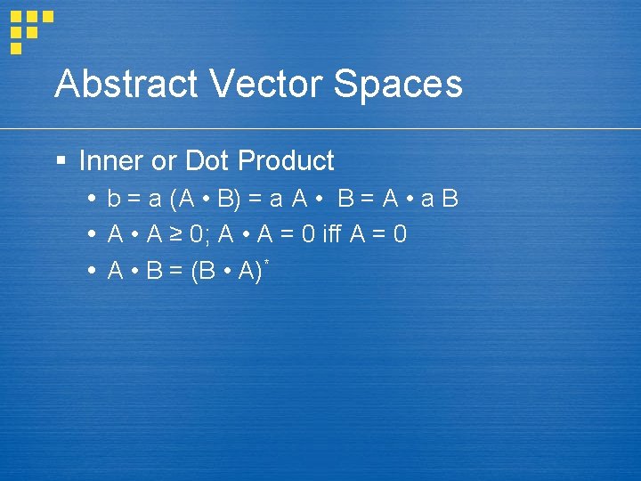
Abstract Vector Spaces § Inner or Dot Product b = a (A • B) = a A • B = A • a B A • A ≥ 0; A • A = 0 iff A = 0 A • B = (B • A)*

Vectors and Discrete Functions Geometric Vector Discrete Function V = (1, 2, 4) V[I] = {1, 2, 4} Linearity a. V+b. U a V[I] + b U[I] Dot Product V • U ∑ (V[I] U*[I]) Vector Interpretation

Vectors and Discrete Functions § 2 t in terms of t 0, t 1, t 2 = [1, . 5] 2 t 1 t t 2

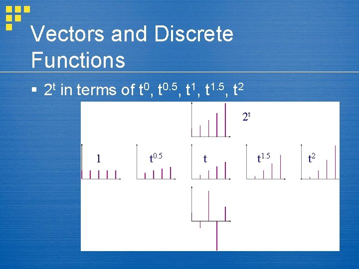
Vectors and Discrete Functions § 2 t in terms of t 0, t 0. 5, t 1. 5, t 2 2 t 1 t 0. 5 t t 1. 5 t 2

Vectors and Functions Vector Discrete Continuous V V[I] V(x) a. V+b. U a V[I] + b U[I] a V(x) + b U(x) V • U ∑ V[I] U*[I] ∫ V(x) U*(x) dx

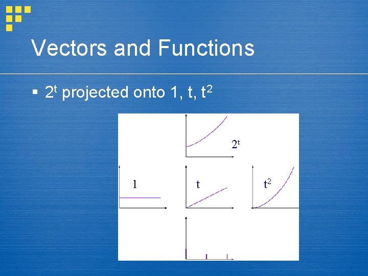
Vectors and Functions § 2 t projected onto 1, t, t 2 2 t 1 t t 2

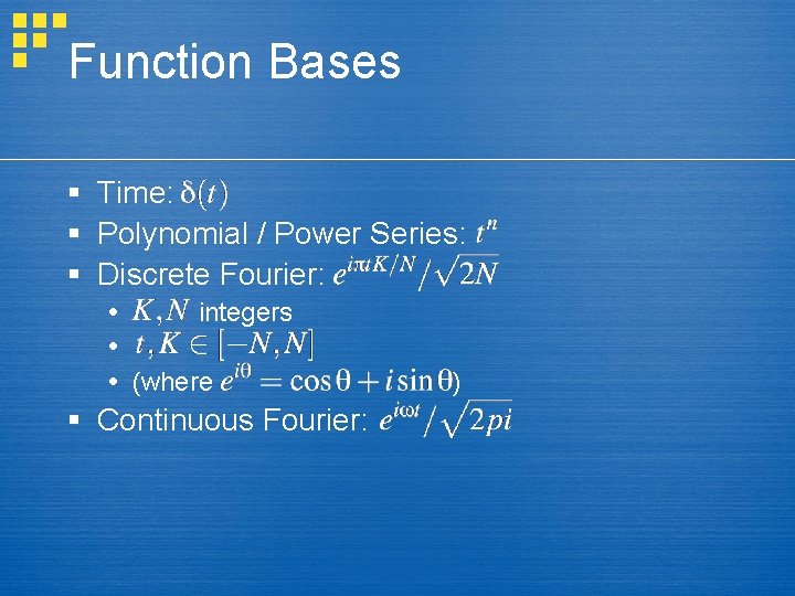
Function Bases § Time: § Polynomial / Power Series: § Discrete Fourier: integers (where § Continuous Fourier: )

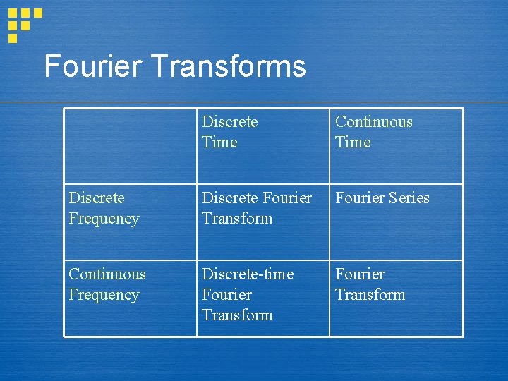
Fourier Transforms Discrete Time Continuous Time Discrete Frequency Discrete Fourier Transform Fourier Series Continuous Frequency Discrete-time Fourier Transform

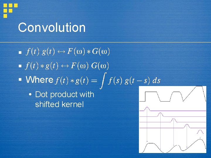
Convolution § § § Where Dot product with shifted kernel

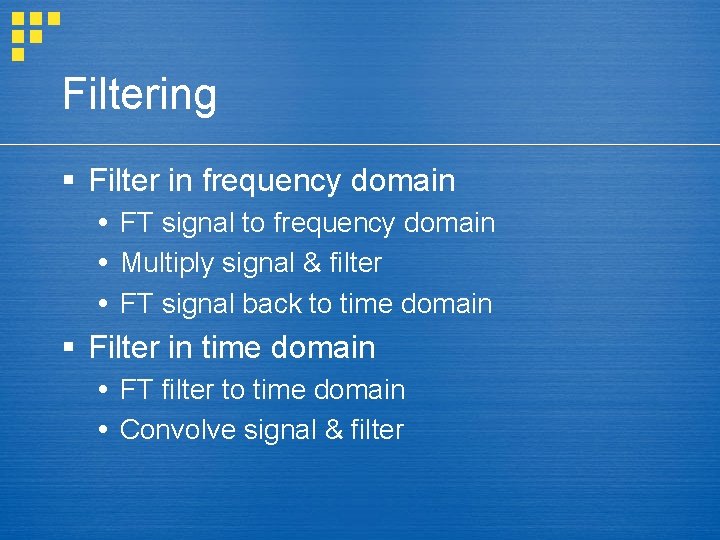
Filtering § Filter in frequency domain FT signal to frequency domain Multiply signal & filter FT signal back to time domain § Filter in time domain FT filter to time domain Convolve signal & filter

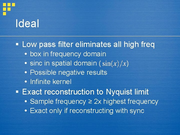
Ideal § Low pass filter eliminates all high freq box in frequency domain sinc in spatial domain ( Possible negative results Infinite kernel ) § Exact reconstruction to Nyquist limit Sample frequency ≥ 2 x highest frequency Exact only if reconstructing with sync

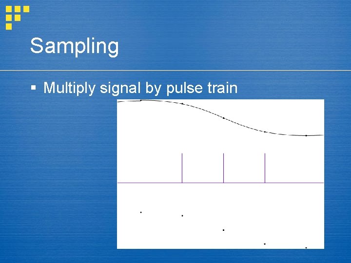
Sampling § Multiply signal by pulse train

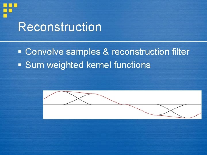
Reconstruction § Convolve samples & reconstruction filter § Sum weighted kernel functions

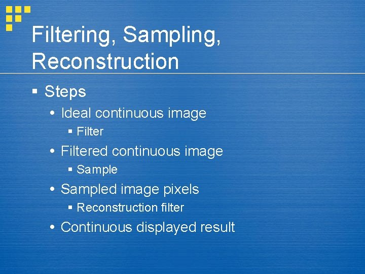
Filtering, Sampling, Reconstruction § Steps Ideal continuous image § Filtered continuous image § Sampled image pixels § Reconstruction filter Continuous displayed result

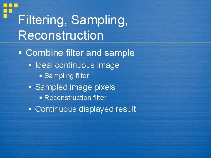
Filtering, Sampling, Reconstruction § Combine filter and sample Ideal continuous image § Sampling filter Sampled image pixels § Reconstruction filter Continuous displayed result

Antialiasing § Blur away frequencies that would alias § Blur preferable to aliasing § Can combine filtering and sampling Evaluate convolution at sample points § Filter kernel size IIR = infinite impulse response FIR = finite impulse response

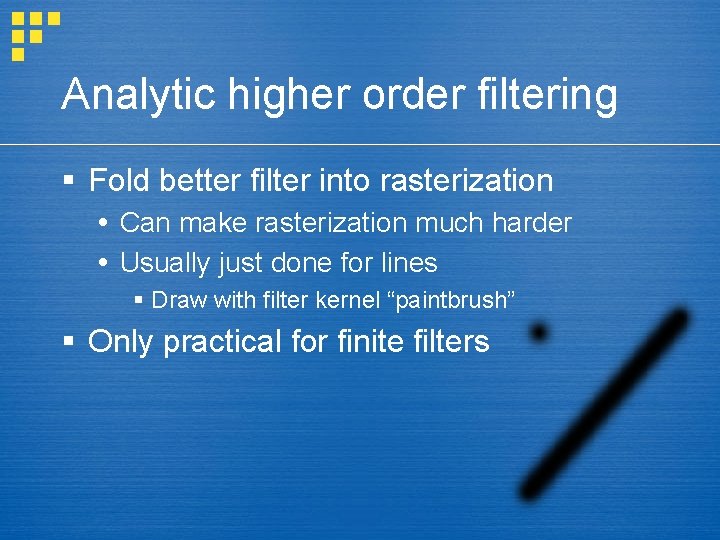
Analytic higher order filtering § Fold better filter into rasterization Can make rasterization much harder Usually just done for lines § Draw with filter kernel “paintbrush” § Only practical for finite filters

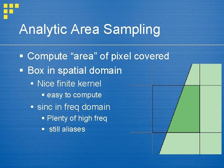
Analytic Area Sampling § Compute “area” of pixel covered § Box in spatial domain Nice finite kernel § easy to compute sinc in freq domain § Plenty of high freq § still aliases

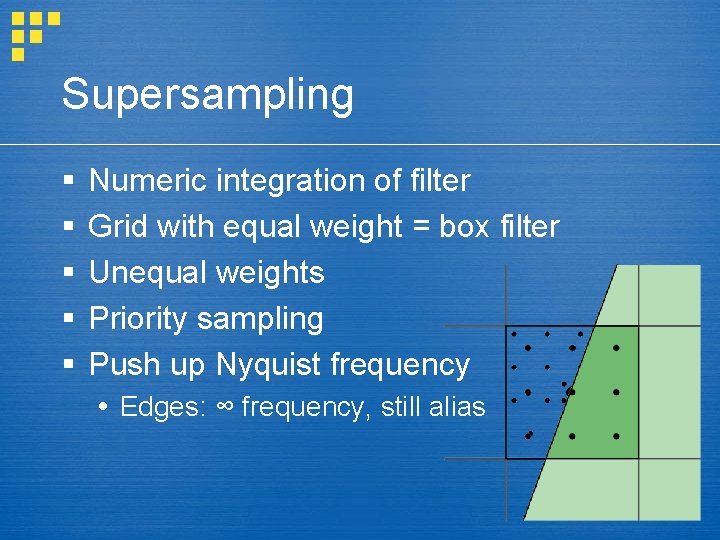
Supersampling § § § Numeric integration of filter Grid with equal weight = box filter Unequal weights Priority sampling Push up Nyquist frequency Edges: ∞ frequency, still alias

Adaptive sampling § § Numerical integration with varying step More samples in high contrast areas Easy with ray tracing, harder for others Possible bias

Stochastic sampling § Monte-Carlo integration of filter § Sample distribution Poisson disk Jittered grid § Aliasing Noise

Which filter kernel? § Finite impulse response Finite filter Windowed filter § Positive everywhere? § Ringing?

Which filter kernel? § Windowed sync § Windowed Gaussian (~0 @ 6 ) § Box, tent, cubic

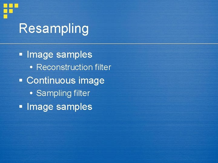
Resampling § Image samples Reconstruction filter § Continuous image Sampling filter § Image samples