Chapter 9 Switching models Introductory Econometrics for Finance

Chapter 9 Switching models ‘Introductory Econometrics for Finance’ © Chris Brooks 2002 1

Switching Models • Motivation: Episodic nature of economic and financial variables. What might cause these fundamental changes in behaviour? - Wars - Financial panics - Significant changes in government policy - Changes in market microstructure - e. g. big bang - Changes in market sentiment - Market rigidities • Switches can be one-off single changes or occur frequently back and forth. ‘Introductory Econometrics for Finance’ © Chris Brooks 2002 2

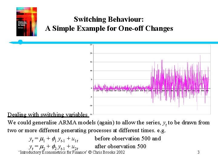
Switching Behaviour: A Simple Example for One-off Changes Dealing with switching variables We could generalise ARMA models (again) to allow the series, yt to be drawn from two or more different generating processes at different times. e. g. yt = 1 + 1 yt-1 + u 1 t before observation 500 and yt = 2 + 2 yt-1 + u 2 t after observation 500 ‘Introductory Econometrics for Finance’ © Chris Brooks 2002 3

How do we Decide where the Switch or Switches take Place? • It may be obvious from a plot or from knowledge of the history of the series. • It can be determined using a model. • It may occur at fixed intervals as a result of seasonalities. • A number of different approaches are available, and are described below. ‘Introductory Econometrics for Finance’ © Chris Brooks 2002 4

Seasonality in Financial Markets • If we have quarterly or monthly or even daily data, these may have patterns in. • Seasonal effects in financial markets have been widely observed and are often termed “calendar anomalies”. • Examples include day-of-the-week effects, open- or close-of-market effect, January effects, or bank holiday effects. • These result in statistically significantly different behaviour during some seasons compared with others. • Their existence is not necessarily inconsistent with the EMH. ‘Introductory Econometrics for Finance’ © Chris Brooks 2002 5

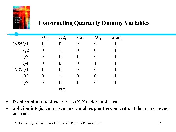
Constructing Dummy Variables for Seasonality • One way to cope with this is the inclusion of dummy variables- e. g. for quarterly data, we could have 4 dummy variables: D 1 t D 2 t D 3 t D 4 t = 1 in Q 1 and zero otherwise = 1 in Q 2 and zero otherwise = 1 in Q 3 and zero otherwise = 1 in Q 4 and zero otherwise • How many dummy variables do we need? We need one less than the “seasonality” of the data. e. g. for quarterly series, consider what happens if we use all 4 dummies ‘Introductory Econometrics for Finance’ © Chris Brooks 2002 6

Constructing Quarterly Dummy Variables 1986 Q 1 Q 2 Q 3 Q 4 1987 Q 1 Q 2 Q 3 D 1 t 1 0 0 0 1 0 0 D 2 t 0 1 0 0 0 1 0 etc. D 3 t 0 0 1 0 0 0 1 D 4 t 0 0 0 1 0 0 0 Sumt 1 1 • Problem of multicollinearity so (X X)-1 does not exist. • Solution is to just use 3 dummy variables plus the constant or 4 dummies and no constant. ‘Introductory Econometrics for Finance’ © Chris Brooks 2002 7

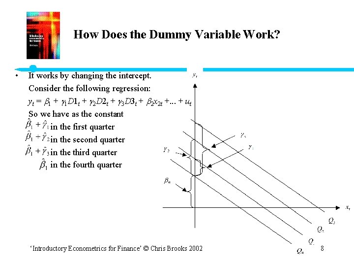
How Does the Dummy Variable Work? • It works by changing the intercept. Consider the following regression: yt = 1 + 1 D 1 t + 2 D 2 t + 3 D 3 t + 2 x 2 t +. . . + ut So we have as the constant in the first quarter in the second quarter in the third quarter in the fourth quarter ‘Introductory Econometrics for Finance’ © Chris Brooks 2002 8

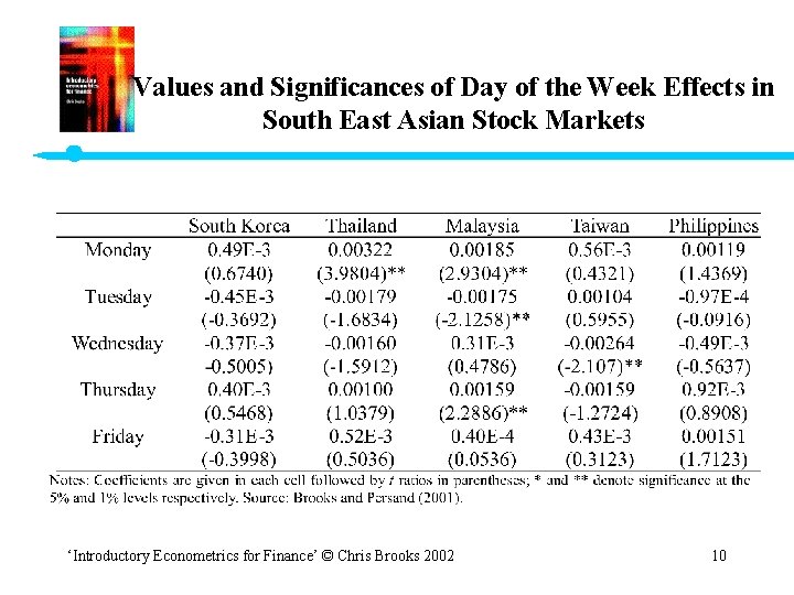
Seasonalities in South East Asian Stock Returns • Brooks and Persand (2001) examine the evidence for a day-of-theweek effect in five Southeast Asian stock markets: South Korea, Malaysia, the Philippines, Taiwan and Thailand. • The data, are on a daily close-to-close basis for all weekdays (Mondays to Fridays) falling in the period 31 December 1989 to 19 January 1996 (a total of 1581 observations). • They use daily dummy variables for the day of the week effects in the regression: rt = 1 D 1 t + 2 D 2 t + 3 D 3 t + 4 D 4 t + 5 D 5 t + ut • Then the coefficients can be interpreted as the average return on each day of the week. ‘Introductory Econometrics for Finance’ © Chris Brooks 2002 9

Values and Significances of Day of the Week Effects in South East Asian Stock Markets ‘Introductory Econometrics for Finance’ © Chris Brooks 2002 10

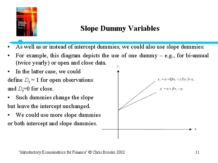
Slope Dummy Variables • As well as or instead of intercept dummies, we could also use slope dummies: • For example, this diagram depicts the use of one dummy – e. g. , for bi-annual (twice yearly) or open and close data. • In the latter case, we could define Dt = 1 for open observations and Dt=0 for close. • Such dummies change the slope but leave the intercept unchanged. • We could use more slope dummies or both intercept and slope dummies. ‘Introductory Econometrics for Finance’ © Chris Brooks 2002 11

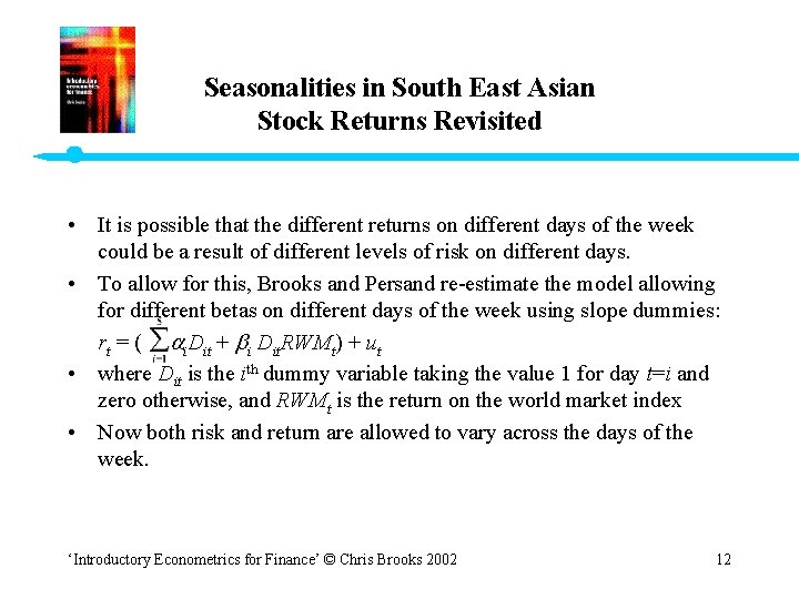
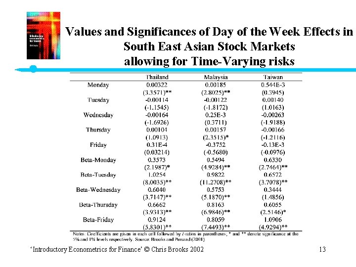
Seasonalities in South East Asian Stock Returns Revisited • It is possible that the different returns on different days of the week could be a result of different levels of risk on different days. • To allow for this, Brooks and Persand re-estimate the model allowing for different betas on different days of the week using slope dummies: rt = ( i. Dit + i Dit. RWMt) + ut • where Dit is the ith dummy variable taking the value 1 for day t=i and zero otherwise, and RWMt is the return on the world market index • Now both risk and return are allowed to vary across the days of the week. ‘Introductory Econometrics for Finance’ © Chris Brooks 2002 12

Values and Significances of Day of the Week Effects in South East Asian Stock Markets allowing for Time-Varying risks ‘Introductory Econometrics for Finance’ © Chris Brooks 2002 13

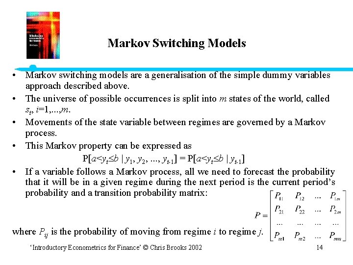
Markov Switching Models • Markov switching models are a generalisation of the simple dummy variables approach described above. • The universe of possible occurrences is split into m states of the world, called st, i=1, . . . , m. • Movements of the state variable between regimes are governed by a Markov process. • This Markov property can be expressed as P[a<yt b y 1, y 2, . . . , yt-1] = P[a<yt b yt-1] • If a variable follows a Markov process, all we need to forecast the probability that it will be in a given regime during the next period is the current period’s probability and a transition probability matrix: where Pij is the probability of moving from regime i to regime j. ‘Introductory Econometrics for Finance’ © Chris Brooks 2002 14

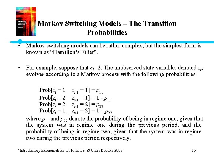
Markov Switching Models – The Transition Probabilities • Markov switching models can be rather complex, but the simplest form is known as “Hamilton’s Filter”. • For example, suppose that m=2. The unobserved state variable, denoted zt, evolves according to a Markov process with the following probabilities Prob[zt = 1 zt-1 = 1] = p 11 Prob[zt = 2 zt-1 = 1] = 1 - p 11 Prob[zt = 2 zt-1 = 2] = p 22 Prob[zt = 1 zt-1 = 2] = 1 – p 22 where p 11 and p 22 denote the probability of being in regime one, given that the system was in regime one during the previous period, and the probability of being in regime two, given that the system was in regime two during the previous period respectively. ‘Introductory Econometrics for Finance’ © Chris Brooks 2002 15

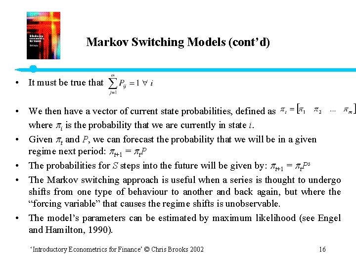
Markov Switching Models (cont’d) • It must be true that • We then have a vector of current state probabilities, defined as where i is the probability that we are currently in state i. • Given t and P, we can forecast the probability that we will be in a given regime next period: t+1 = t. P • The probabilities for S steps into the future will be given by: t+1 = t. Ps • The Markov switching approach is useful when a series is thought to undergo shifts from one type of behaviour to another and back again, but where the “forcing variable” that causes the regime shifts is unobservable. • The model’s parameters can be estimated by maximum likelihood (see Engel and Hamilton, 1990). ‘Introductory Econometrics for Finance’ © Chris Brooks 2002 16

An Application of Markov Switching Models to the Gilt-Equity Yield Ratio • The gilt-equity yield ratio (GEYR) is defined as the ratio of the income yield on long-term government bonds to the dividend yield on equities. • It has been suggested that the current value of the GEYR might be a useful tool for investment managers or market analysts • The GEYR is assumed to have a long-run equilibrium level, deviations from which are taken to signal that equity prices are at an unsustainable level. • Thus, in its crudest form, an equity trading rule based on the GEYR would say, “if the GEYR is low, buy equities; if the GEYR is high, sell equities. ” • Brooks and Persand (2001) employ monthly stock index dividend yields and income yields on government bonds covering the period January 1975 until August 1997 (272 observations) for three countries - the UK, the US, and Germany. ‘Introductory Econometrics for Finance’ © Chris Brooks 2002 17

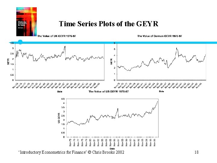
Time Series Plots of the GEYR ‘Introductory Econometrics for Finance’ © Chris Brooks 2002 18

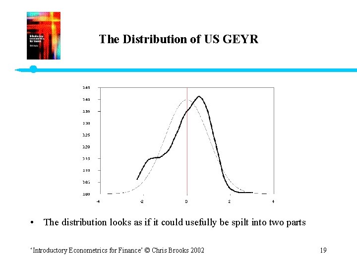
The Distribution of US GEYR • The distribution looks as if it could usefully be spilt into two parts ‘Introductory Econometrics for Finance’ © Chris Brooks 2002 19

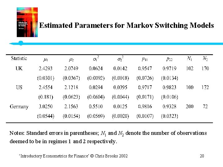
Estimated Parameters for Markov Switching Models Notes: Standard errors in parentheses; N 1 and N 2 denote the number of observations deemed to be in regimes 1 and 2 respectively. ‘Introductory Econometrics for Finance’ © Chris Brooks 2002 20

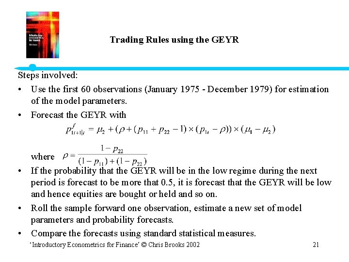
Trading Rules using the GEYR Steps involved: • Use the first 60 observations (January 1975 - December 1979) for estimation of the model parameters. • Forecast the GEYR with where • If the probability that the GEYR will be in the low regime during the next period is forecast to be more that 0. 5, it is forecast that the GEYR will be low and hence equities are bought or held and so on. • Roll the sample forward one observation, estimate a new set of model parameters and probability forecasts. • Compare the forecasts using standard statistical measures. ‘Introductory Econometrics for Finance’ © Chris Brooks 2002 21

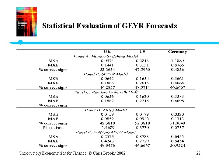
Statistical Evaluation of GEYR Forecasts ‘Introductory Econometrics for Finance’ © Chris Brooks 2002 22

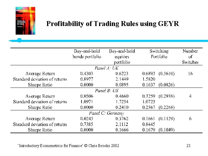
Profitability of Trading Rules using GEYR ‘Introductory Econometrics for Finance’ © Chris Brooks 2002 23

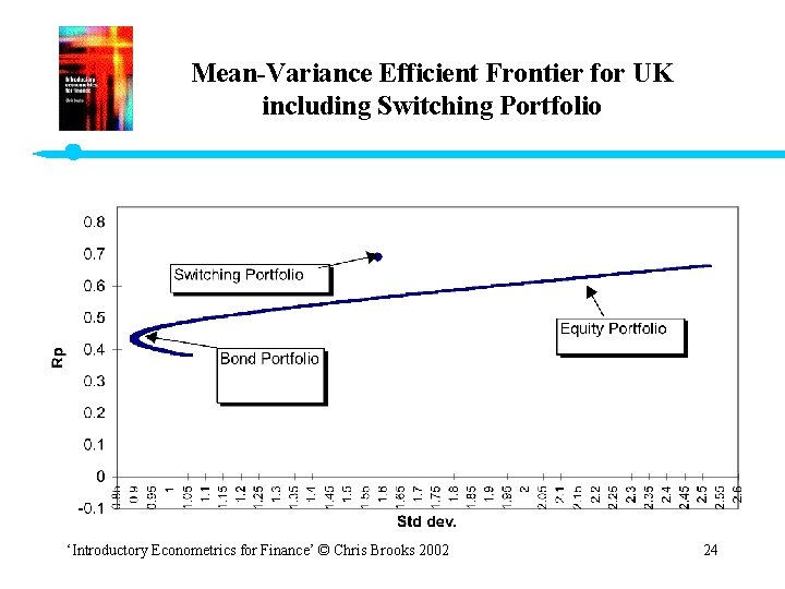
Mean-Variance Efficient Frontier for UK including Switching Portfolio ‘Introductory Econometrics for Finance’ © Chris Brooks 2002 24

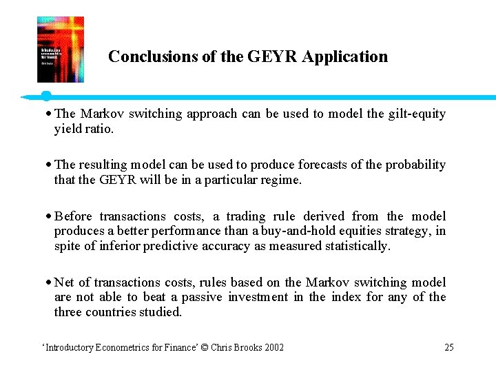
Conclusions of the GEYR Application · The Markov switching approach can be used to model the gilt-equity yield ratio. · The resulting model can be used to produce forecasts of the probability that the GEYR will be in a particular regime. · Before transactions costs, a trading rule derived from the model produces a better performance than a buy-and-hold equities strategy, in spite of inferior predictive accuracy as measured statistically. · Net of transactions costs, rules based on the Markov switching model are not able to beat a passive investment in the index for any of the three countries studied. ‘Introductory Econometrics for Finance’ © Chris Brooks 2002 25

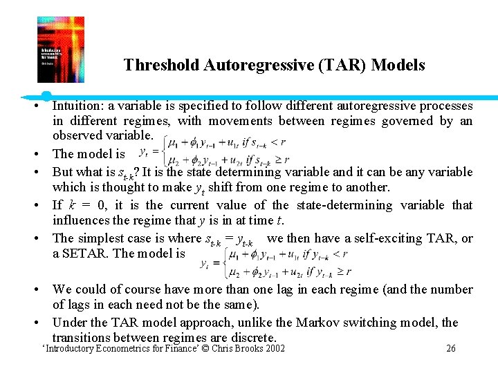
Threshold Autoregressive (TAR) Models • Intuition: a variable is specified to follow different autoregressive processes in different regimes, with movements between regimes governed by an observed variable. • The model is • But what is st-k? It is the state determining variable and it can be any variable which is thought to make yt shift from one regime to another. • If k = 0, it is the current value of the state-determining variable that influences the regime that y is in at time t. • The simplest case is where st-k = yt-k we then have a self-exciting TAR, or a SETAR. The model is • We could of course have more than one lag in each regime (and the number of lags in each need not be the same). • Under the TAR model approach, unlike the Markov switching model, the transitions between regimes are discrete. ‘Introductory Econometrics for Finance’ © Chris Brooks 2002 26

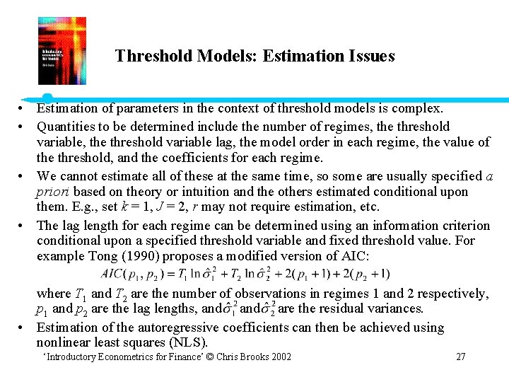
Threshold Models: Estimation Issues • Estimation of parameters in the context of threshold models is complex. • Quantities to be determined include the number of regimes, the threshold variable lag, the model order in each regime, the value of the threshold, and the coefficients for each regime. • We cannot estimate all of these at the same time, so some are usually specified a priori based on theory or intuition and the others estimated conditional upon them. E. g. , set k = 1, J = 2, r may not require estimation, etc. • The lag length for each regime can be determined using an information criterion conditional upon a specified threshold variable and fixed threshold value. For example Tong (1990) proposes a modified version of AIC: where T 1 and T 2 are the number of observations in regimes 1 and 2 respectively, p 1 and p 2 are the lag lengths, and are the residual variances. • Estimation of the autoregressive coefficients can then be achieved using nonlinear least squares (NLS). ‘Introductory Econometrics for Finance’ © Chris Brooks 2002 27

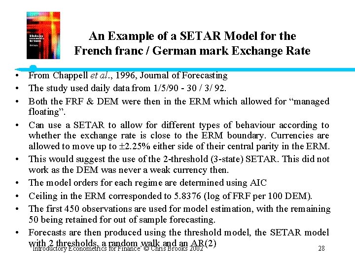
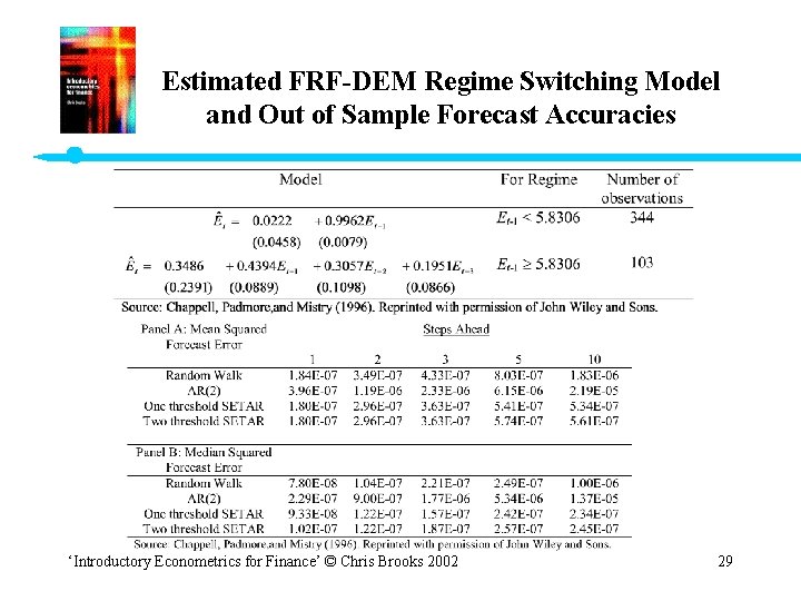
An Example of a SETAR Model for the French franc / German mark Exchange Rate • From Chappell et al. , 1996, Journal of Forecasting • The study used daily data from 1/5/90 - 30 / 3/ 92. • Both the FRF & DEM were then in the ERM which allowed for “managed floating”. • Can use a SETAR to allow for different types of behaviour according to whether the exchange rate is close to the ERM boundary. Currencies are allowed to move up to 2. 25% either side of their central parity in the ERM. • This would suggest the use of the 2 -threshold (3 -state) SETAR. This did not work as the DEM was never a weak currency then. • The model orders for each regime are determined using AIC • Ceiling in the ERM corresponded to 5. 8376 (log of FRF per 100 DEM). • The first 450 observations are used for model estimation, with the remaining 50 being retained for out of sample forecasting. • Forecasts are then produced using the threshold model, the SETAR model with 2 thresholds, a random walk and an AR(2) ‘Introductory Econometrics for Finance’ © Chris Brooks 2002 28

Estimated FRF-DEM Regime Switching Model and Out of Sample Forecast Accuracies ‘Introductory Econometrics for Finance’ © Chris Brooks 2002 29