Chapter 1 Linear Functions Slopes and Equations of

Chapter 1 Linear Functions

Slopes and Equations of Lines l The Rectangular Coordinate System – – – The horizontal number line is the x-axis The vertical number line is the y-axis The point where the axes intersect is the origin (the 0 point)

Slopes and Equations of Lines l The point given as (2, 3) is also called an ordered pair. – – Where 2 is the x coordinate, the first coordinate, the abscissa, or the horizontal distance Where 3 is the y coordinate, the second coordinate, the ordinate, or the vertical distance

Slopes and Equations of Lines l Intercepts of a Line – – The y-intercept of a line is the point (0, b) where the line intersects the y axis. To find b, substitute 0 for x in the equation of the line and solve for y. The x-intercept of a line is the point (a, 0) where the line intersects the x-axis. To find a, substitute 0 for y in the equation of a line and solve for x.

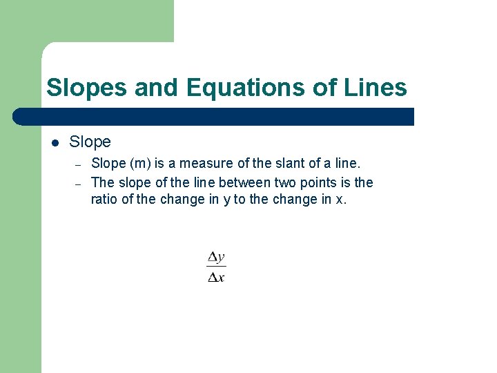
Slopes and Equations of Lines l Slope – – Slope (m) is a measure of the slant of a line. The slope of the line between two points is the ratio of the change in y to the change in x.

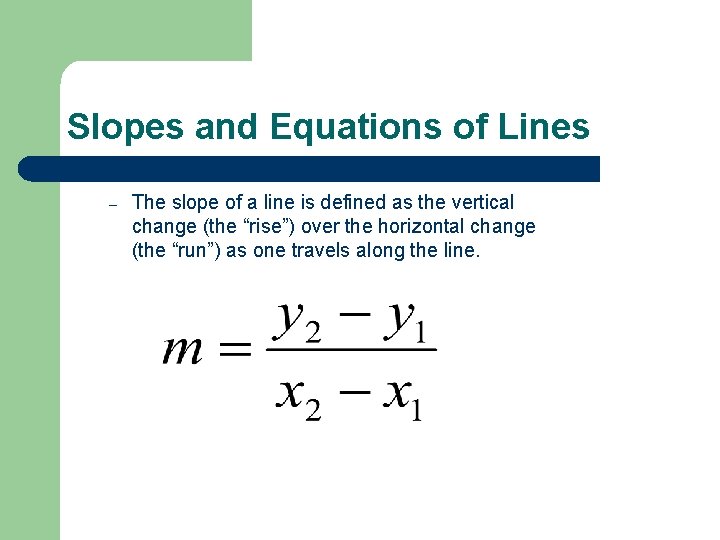
Slopes and Equations of Lines – The slope of a line is defined as the vertical change (the “rise”) over the horizontal change (the “run”) as one travels along the line.

Slopes and Equations of Lines l Slope of a Line

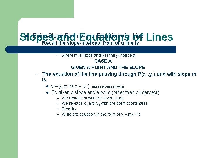
l Point-Slope Form of the Equation of a Line Slopes and Equations of Lines Recall the slope-intercept from of a line is – l Y = mx + b – where m is slope and b is the y-intercept CASE A GIVEN A POINT AND THE SLOPE – The equation of the line passing through P(x 1, y 1) and with slope m is l l y – y 1 = m( x – x 1 ) (the point-slope formula) So given a slope and a point (other than y-intercept) – We replace m with the given slope – We replace x 1 and y 1 with the point coordinates – Simplify – Write the equation in the form of y = mx + b

Slopes and Equations of Lines CASE B GIVEN TWO POINTS ONLY – The equation of the line passing through P(x 1, y 1) and P(x 2, y 2) (slope is not given) l l We first use the slope formula to determine slope Then we use one of the given points and the slope in the pointslope formula y – y 1 = m( x – x 1 )

Slopes and Equations of Lines CASE C GIVEN A POINT P(x 1, y 1) AND AN UNDEFINED SLOPE – – – Recall that a line with an undefined slope is a vertical line with x = a, where a is the x-coordinate of the x-intercept (x 1, 0) Recall that for a vertical line, the x-coordinate doesn’t change. the equation would simply be x = x 1

Slopes and Equations of Lines CASE D GIVEN A POINT P(x 1, y 1) AND A ZERO SLOPE – – – Recall that a line with a zero slope is a horizontal line with y = b, where b is the y-coordinate of the y -intercept (0, b) Recall that for a horizontal line, the y-coordinate doesn’t change. the equation would simply be y = y 1

Slopes and Equations of Lines CASE E GIVEN THE Y-INTERCEPT (0, b) AND SLOPE – We use the slope-intercept form l y = mx +b Replace m with the given slope – Replace b with the given y-coordinate –

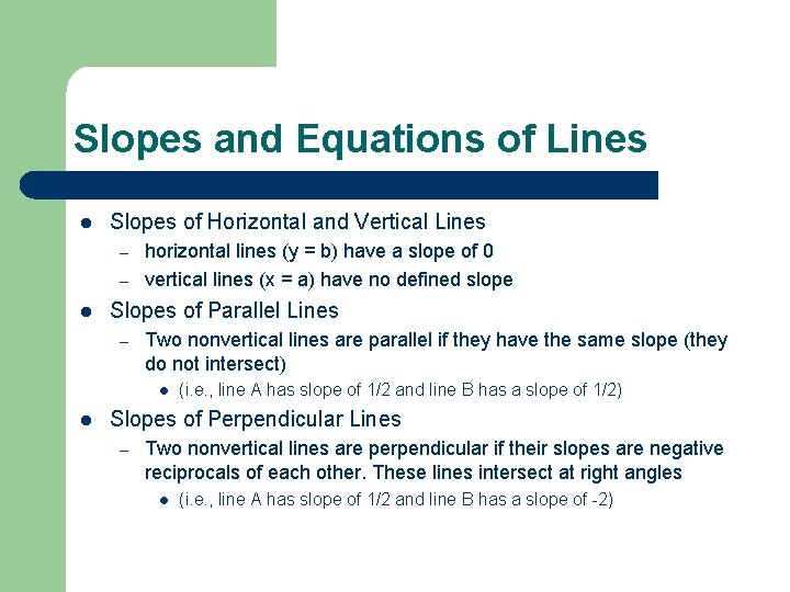
Slopes and Equations of Lines l Slopes of Horizontal and Vertical Lines – – l horizontal lines (y = b) have a slope of 0 vertical lines (x = a) have no defined slope Slopes of Parallel Lines – Two nonvertical lines are parallel if they have the same slope (they do not intersect) l l (i. e. , line A has slope of 1/2 and line B has a slope of 1/2) Slopes of Perpendicular Lines – Two nonvertical lines are perpendicular if their slopes are negative reciprocals of each other. These lines intersect at right angles l (i. e. , line A has slope of 1/2 and line B has a slope of -2)

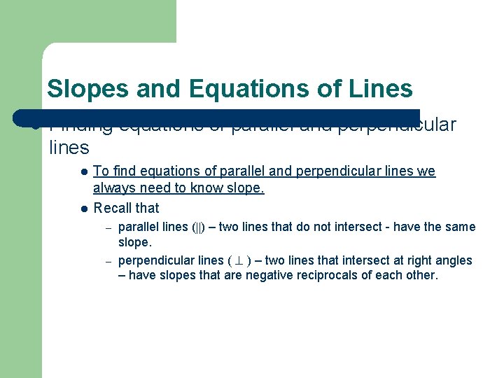
Slopes and Equations of Lines l Finding equations of parallel and perpendicular lines l l To find equations of parallel and perpendicular lines we always need to know slope. Recall that parallel lines ( ) – two lines that do not intersect - have the same slope. – perpendicular lines ( ) – two lines that intersect at right angles – have slopes that are negative reciprocals of each other. –

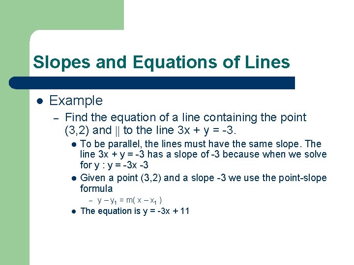
Slopes and Equations of Lines l Example – Find the equation of a line containing the point (3, 2) and to the line 3 x + y = -3. l l To be parallel, the lines must have the same slope. The line 3 x + y = -3 has a slope of -3 because when we solve for y : y = -3 x -3 Given a point (3, 2) and a slope -3 we use the point-slope formula – l y – y 1 = m( x – x 1 ) The equation is y = -3 x + 11

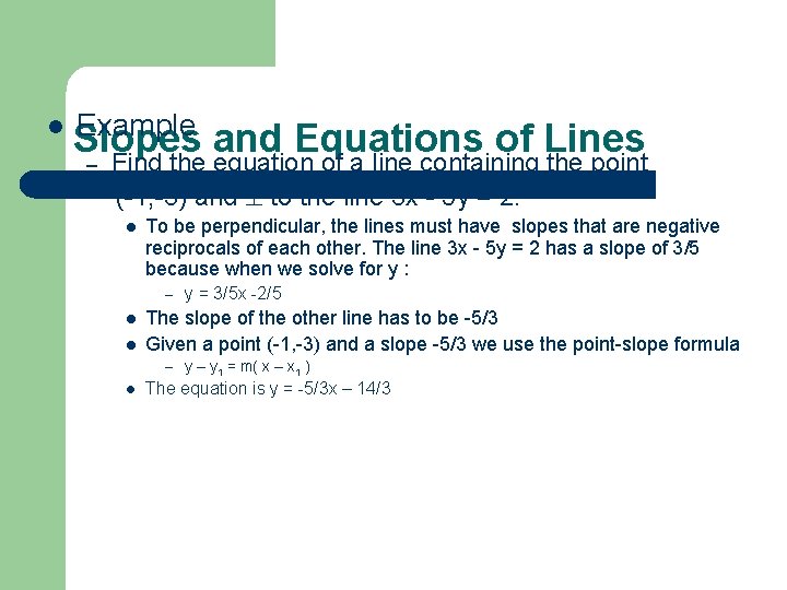
l Example Slopes and Equations of Lines – Find the equation of a line containing the point (-1, -3) and to the line 3 x - 5 y = 2. l To be perpendicular, the lines must have slopes that are negative reciprocals of each other. The line 3 x - 5 y = 2 has a slope of 3/5 because when we solve for y : – l l y = 3/5 x -2/5 The slope of the other line has to be -5/3 Given a point (-1, -3) and a slope -5/3 we use the point-slope formula – y 1 = m( x – x 1 ) l The equation is y = -5/3 x – 14/3

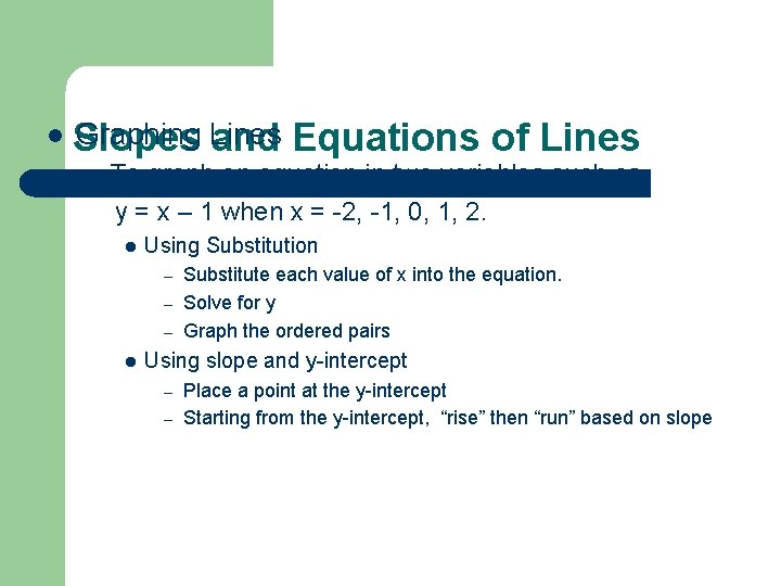
l Graphing Lines Slopes and Equations of Lines – To graph an equation in two variables such as y = x – 1 when x = -2, -1, 0, 1, 2. l Using Substitution Substitute each value of x into the equation. – Solve for y – Graph the ordered pairs – l Using slope and y-intercept Place a point at the y-intercept – Starting from the y-intercept, “rise” then “run” based on slope –

Linear Functions And Applications l Linear Functions – Notation – f(x) l – Note: f, g, or h are often used to name functions The function f(x) is defined by l y = f(x) = mx + b

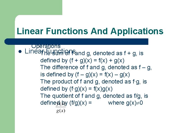
Linear Functions And Applications Operations l Linear Functions The sum of f and g, denoted as f + g, is defined by (f + g)(x) = f(x) + g(x) The difference of f and g, denoted as f – g, is defined by (f – g)(x) = f(x) – g(x) The product of f and g, denoted as f∙g, is defined by (f∙g)(x) = f(x)g(x) The quotient of f and g, denoted as f/g, is defined by (f/g)(x) = where g(x) 0

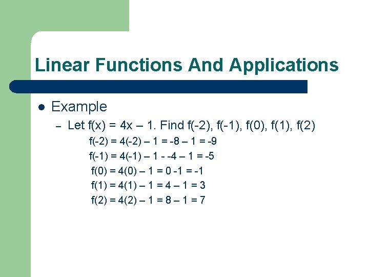
Linear Functions And Applications l Example – Let f(x) = 4 x – 1. Find f(-2), f(-1), f(0), f(1), f(2) f(-2) = 4(-2) – 1 = -8 – 1 = -9 f(-1) = 4(-1) – 1 - -4 – 1 = -5 f(0) = 4(0) – 1 = 0 -1 = -1 f(1) = 4(1) – 1 = 4 – 1 = 3 f(2) = 4(2) – 1 = 8 – 1 = 7

Linear Functions And Applications l Supply and Demand – Supply and Demand functions are not necessarily linear l – Most approximately linear Equilibrium Price/Quantity l l Equilibrium price of a commodity is the price found at the point where the supply and demand are equal (i. e. , where the supply and demand graphs for that commodity intersect). Equilibrium quantity is the quantity where the prices from both demand the supply are equal.

Linear Functions And Applications l Cost Analysis – The cost of manufacturing an item commonly consists of two parts: l Fixed cost – designing the product, setting up a factory, training workers, etc. l Marginal cost – approximates the cost of producing one additional item.

Linear Functions And Applications l Cost Analysis – The Cost Function l C(x) = mx + b where m represents marginal cost per item where b represents the fixed cost

Linear Functions And Applications l Break-Even Analysis – – – Involves both revenue and profit. Revenue R(x) = px where p represents the price per unit of product where x represents the number of units sold (demand) Profit P(x) is the difference between revenue and cost: l l l P(x) = R(x) – C(x) Break-even quantity – the number of units at which revenue just equals cost Break-even point – the point where revenue equals cost.

The Least Squares Line l In practice, how are equations of supply and demand functions found? – – Data is collected Data is plotted l l Data lie perfectly along a line – equation easily found using any two points Data scattered and no line that goes through all points – must find a line that approximates the linear trend of the data as closely as possible (Method of Least Squares)

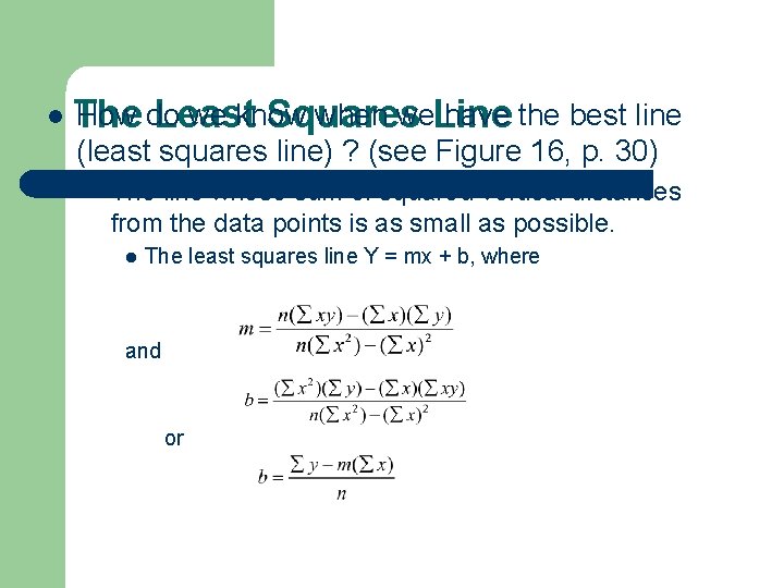
l How do we know when we. Line have the best line The Least Squares (least squares line) ? (see Figure 16, p. 30) – The line whose sum of squared vertical distances from the data points is as small as possible. l The least squares line Y = mx + b, where and or

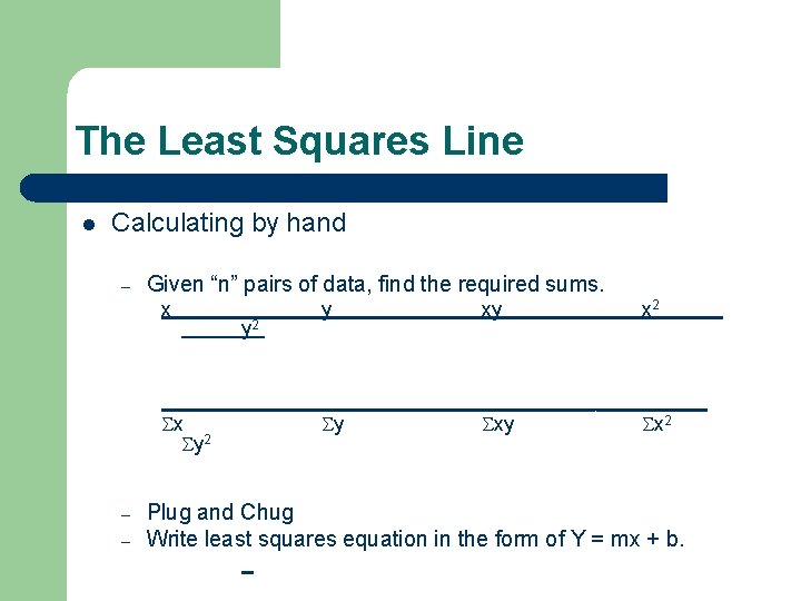
The Least Squares Line l Calculating by hand – Given “n” pairs of data, find the required sums. x y 2 y xy x 2 _________________________ x y xy x 2 y 2 – – Plug and Chug Write least squares equation in the form of Y = mx + b.

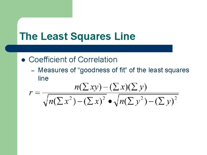
The Least Squares Line l Coefficient of Correlation – Measures of “goodness of fit” of the least squares line

The Least Squares Line – – – The coefficient of correlation (r) is always equal to or between 1 and -1. Coefficient of correlation (r) values of exactly 1 or -1 mean that the data points lie exactly on the least squares line. If r = 1, the least squares line has a positive slope If r = -1, the least squares line has a negative slope If r = 0, there is no linear correlation between the data points (some nonlinear function might provide a better fit) The closer the value of r is to 1 or -1, the stronger the linear relationship between the data points.