Centimeter Receiver Design Considerations with a look to

Centimeter Receiver Design Considerations with a look to the future Steven White National Radio Astronomy Observatory Green Bank, WV

Todd. Hunter, Fred. Schwab. GBT High-Frequency Efficiency Improvements, NRAO May 2009 Newsletter

Performance Limitations • Surface (Ruze λ/16) – – ξ = 50% 300 µmeters → 63 Ghz • Atmosphere e-t t = optical depth • Spill Over Ts • Pointing • Receiver Noise Temperature (Amplifier) TR

Frequency Coverage • 300 Mhz to 90 Ghz • l: 1 meter to 3 millimeters • l < 1/3 meter - Gregorian Focus • l > 1/3 meter - Prime Focus

Gregorian Subreflector

Prime Focus Feed Cross Dipole 290 -395 MHz

Reflector Feeds Profile: L (size), S (size), Ka (spacing), KFPA (spacing), Q (spacing) Linear Taper: C, X, Ku, K Design Parameters: Length (Bandwidth), Aperture (Taper, Efficiency) GBT α= 15º , Focal Length = 15. 1 meters, Dimensions = 7. 55 x 7. 95 meters

Optimizing G/T

Gregorian Feeds S, Ku (2 x), L W band feed KFPA Feed 140’ Prime Focus and Cassegrain Feed 140’ & 300’ Hybrid mode prime focus

Radio Source Properties • Total Power (continuum: cmb, dust) – Correlation Radiometer Receivers (Ka Band) – Bolometers Receivers (MUSTANG) • Frequency Spectrum (spectral line, redshifts, emission, absorption) – Hetrodyne – Prime 1 & 2, L, S, C, X, Ku, K, Ka, Q • Polarization (magnetic fields) – Requires OMT – Limits Bandwidth • Pulse Profiles (Pulsars) • Very Long Baseline Interferometry (VLBI) – Phase Calibration

Prime Focus Receiver • PF 1. 1 • PF 1. 2 • PF 1. 3 • PF 1. 4 • PF 2 Frequency 0. 290 - 0. 395 0. 385 - 0. 520 0. 510 - 0. 690 0. 680 - 0. 920 0. 910 - 1. 230 Trec 12 22 12 21 10 Tsys 46 K 43 K 22 K 29 K 17 K Feed X Dipole Linear Taper

Gregorian Receivers Frequency Band [GHz] • • • 1 -2 L 2 -3 S 4 -6 C 8 -10 X 12 -15 Ku 18 -25 K 22 -26 K 26 -40 Ka 40 -52 Q 80 -100 W Wave Guide Band [GHz] OMT (Septum) 12. 4 -18. 0 - 26. 5 - 40. 0 33 - 50. 0 75 to 110 Temperature [º K] Trec Tsys 6 8 -12 5 13 14 21 21 20 40 -70 20 22 18 27 30 30 -40 35 -45 67 -134 ~ 3 10^-16 W/√Hz

Receiver Room Turret

Receiver Room Inside

Polarization Measurements • Linear – Ortho Mode Transducer – Separates Vertical and Horizontal • Circular – OMT + Phase Shifter (limits bandwidth) – 45 Twist – Or 90 Hybrid to generate circular from linear

Linear Polarization Orthomode Transducer

Circular Polarization

A Variety of OMTs

K band OMT

Equivalent Noise

Amplifier Equivalent Noise

Amplifier Cascade

Input Losses

HFET Noise Temperature

Radiometer

Correlation Radiometer (Ka/WMAP)

1/f Amplifier Noise

MUSTANG 1/f Noise

HEMT 1/f Chop Rates Amplifier νo [GHz] (band) Δνrf [GHz] fchop(ε =. 1) [Hz] Δνrf (ε =. 1, f = 5 Hz) [GHz] L 1. 5 0. 8 3 C 4. 0 1 2 2 X 10 3 7 2 Ka 30 10 80 0. 6 Q 45 15 375 0. 2 W 90 30 1500 0. 1 E. J. Wollack. “High-electron-mobility-transistor gain stability and its design implications for wide band millimeter wave receivers”. Review of Sci. Instrum. 66 (8), August 1995.

A HFET LNA

K-band Map Amplifier

Typical Hetrodyne Receiver

Frequency Conversion

Linearity

Intermodulation

Some GBT Receivers K band Q band

Ka Band

Receiver Testing Digitial Continuum Receiver Lband XX (2) and YY (4)

Ku Band Refrigerator Modulation

Ka Receiver (Correlation) Zpectrometer

Lab Spectrometer Waterfall Plot

MUSTANG Bolometer

Focal Plane Array Challenges • • Data Transmission ( State of the Art) Spectrum Analysis ( State of the Art) Software Pipeline Mechanical and Thermal Design. – Packaging – Weight – Maintenance – Cryogenics

Focal Plane Array Algorithm • • Construct Science Case/Aims System Analysis, Cost and Realizability Revaluate Science Requirements → Compromise Instrument Specifications. – Polarization – Number of Pixels – Bandwidth – Resolution

K band Focal Plane Array • Science Driver → Map NH 3 – Polarized without Rotation • Seven Beams → Limited by IF system • 1. 8 GHz BW → Limited by IF system • 800 MHz BW → Limited by Spectrometer

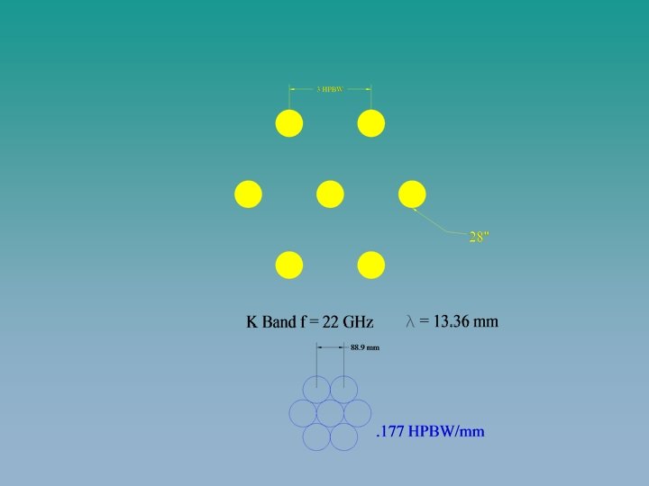
Focal Plane Coverage 1. Initial 7 elements above 68% beam efficiency (illumination and spillover) 2. Expandable to as many as 61 elements 3. beam efficiency of outermost elements would drop to ~60%. 4. beam spacing = 3 HPBWs simulated beam efficiency vs. offset from center

KBand Focal Plane Array

K Band Single Pixel Feed Thermal Transition Phase Shifter Isolators OMT Noise Module HEMT Sliding Transition

Seven Pixel

What’s next for the GBT? • • A W band focal plane array Science Case is strong and under development. Surface is improving Precision Telescope Control System program is improving the servo system. • Needs. – Digital IF system – Backend (CICADA) – Funding (Collaborators)

References • Jarosik, et al. “Design, Implementation and Testing of the MAP Radiometers”, N. The Astrophysical Journal Supplement, 2003, 145 • E. J. Wollack. “High-electron-mobility-transistor gain stability and its design implications for wide band millimeter wave receivers”. Review of Sci. Instrum. 66 (8), August 1995. • M. W. Pospieszalski, “Modeling of Noise Parameters of MESFET’s and MODFET’s and Their Frequency and Temperature Dependence. ” IEEE Trans. MW Theory and Tech. , Vol 37. No. 9 • Norrod and Srikanth, “A Summary of GBT Optics Design”. GBT Memo 155. • Wollack. “A Full Waveguide Band Orthomode Junction. ” NRAO EDIR 303. • • https: //safe. nrao. edu/wiki/bin/view/GB/Knowledge/GBTMemos https: //safe. nrao. edu/wiki/bin/view/Kbandfpa/Web. Home

Thank you for you attention! • Questions?