Categorical Data Analysis Midterm Review Val Aly April

Categorical Data Analysis Midterm Review Val & Aly April 2014

Overview • Regression Analysis: – Mediation – Moderation • Non-parametric tests – When? Why? How?

Example 1 Bumble wants to know whether the relationship between children’s negative affect and self esteem can be explained by children’s bad behavior. Unfortunately, he had to take another vacation to Hawaii, so he left before he could check his results. It’s up to you to do it for him. What do you need to test for?

Mediation Model (Baron & Kenney) M a b c' X Y c

Mediation • Definition: – The mediator (M) explains or accounts for the relationship between X & Y • How to test (packet 2, p. 3) – Baron & Kenney Procedure – Sobel test (obsolete) – Bootstrapping • Interpretation – Avoid causal language, instead say: • “The pattern of correlations is consistent with mediation. ” • “The association between X & Y is mediated by M.

Mediation • Is there evidence for mediation? • Path A: Negative affect Bad behavior B =. 024, p <. 001 • Path B: Bad behavior Self Esteem B = -. 649, p =. 024 • Path C: Negative affect Self Esteem C: B = -. 111, p <. 001 C' : B = -. 096, p <. 001

Moderation Model Moderator X Y

Moderation • Definition – The strength of the relationship between X on Y depends on the level of “Z (Moderator)”. • How to test (packet 3, p. 6) – Multiple regression analysis with an interaction term (X*Moderator) • Interpretation – The association between X and Y is stronger for Z=0 than for Z=1 – Direction and magnitude

Would the association between stress and anxiety differ depending on self-concept complexity? (not complex=0, complex=1) Coefficientsa Standard ized Unstandardized Coefficients Collinearity nts Correlations Std. Model 1 B (Constant) -. 650 . 297 . 339 . 072 Self. Esteem -. 062 . 063 (Constant) -1. 435 . 393 . 154 . 074 -. 031 Beta t Sig. order Toleran Partial Part ce VIF . 030 . 370 4. 700 . 000 . 375 . 371 . 370 . 996 1. 004 -. 078 -. 985 . 326 -. 100 -. 084 -. 077 . 996 1. 004 -3. 648 . 000 . 168 2. 082 . 039 . 375 . 176 . 149 . 789 1. 268 . 058 -. 039 -. 545 . 587 -. 100 -. 047 -. 039 . 987 1. 013 . 181 . 056 . 246 3. 256 . 001 . 364 . 269 . 233 . 900 1. 112 Complexity -. 284 . 068 -. 327 -4. 152 . 000 -. 446 -. 335 -. 297 . 829 1. 207 (Constant) -1. 057 . 411 -2. 572 . 011 . 123 . 073 . 134 1. 677 . 096 . 375 . 143 . 118 . 768 1. 302 -. 028 . 056 -. 035 -. 490 . 625 -. 100 -. 042 -. 034 . 986 1. 014 . 103 . 062 . 140 1. 664 . 098 . 364 . 142 . 117 . 694 1. 442 -. 648 . 154 -. 746 -4. 207 . 000 -. 446 -. 340 -. 295 . 156 6. 395 . 078 . 030 . 442 2. 625 . 010 -. 230 . 220 . 184 . 174 5. 755 GPA Self. Esteem Stress 3 Zero-2. 190 GPA 2 Error Statistics GPA Self. Esteem Stress Complexity Stressx. Complexity a. Dependent Variable: Anxiety level during exam

Anxiety level during exam = -1. 057 +. 123 GPA -. 028 self-esteem +. 103 stress -. 648 complexity +. 078 stress*complexity For people who have complex self-concept, Anxiety level during exam = -1. 057 +. 123 GPA -. 028 self-esteem +. 103 stress -. 648 (1) +. 078 stress*(1) = -1. 705 +. 123 GPA -. 028 self-esteem +. 181 stress For people have simple self-concept, Anxiety level during exam = -1. 057 +. 123 GPA -. 028 self-esteem +. 103 stress -. 648 (0) +. 078 stress*(0) = -1. 057 +. 123 GPA -. 028 self-esteem +. 103 stress Interpretation: Two-way interaction of stress and self-concept complexity was significant. (beta=. 442, p =. 010) This suggests that while holding GPA and self-esteem constant, higher stress is associated with more test anxiety for people with a complex self-concept than those with a simple self-concept.

Non-parametric vs. Parametric tests • Assumptions for parametrics/non-parametrics • Evaluating different measures • Weakness & Benefits • You should argue why you choose one test over the other test (compare two tests & reasons for choice)

Non-parametric analysis Why & When is non-parametric analysis used? (1)When data & distribution do not meet the assumptions of parametric analysis, →normality violation (outlier or skew) →Homogeneity of Variances (check skew & kurtosis, don’t trust Levene) Issues with Levene’s test as a test of homogeneity of variances: Levene’s test is not sensitive enough with small N; even though Levene is n. s. , variances might actually differ enough to be a problem. With very large N, Levene may be significant but the difference in variance may not matter. →with small N, we cannot be confident that the sample represents the population well and cannot assess assumption of normality in the population. (2) When parametric tests are not appropriate →non-parametric tests may be more powerful

Non-parametric tests • Comparing two independent groups (p. 8 – 9, 16 – 17) – Wilcoxon Ws – Mann-Whitney U – Median Test • Comparing two dependent groups (p. 18 – 22) – Wilcoxon T • Contingency Table Statistics (p. 24) – Pearson Chi-squared – Fisher’s exact Test – Mc. Nemar’s test • Variety of Statistics of Effect Size & Correlations (p. 25 – 26) – Kappa – Lambda – Phi – Gamma – Spearman : r : : Wilcoxon : t • Other non-parametric tests (p. 38) – Run’s Test

Which test would you use? 1. To test if 2 variables are independent Non parametric test: Chi Square, Fisher’s exact test (fe <5) Parametric equivalent: Pearson’s r 2. To test the difference between 2 independent groups Non parametric: Wilcoxon W, Mann Whitney U Parametric equivalent: Independent t-test 3. To test the difference between 2 matched groups Non parametric: Wilcoxon T Parametric equivalent: Matched samples t-test

Example Intervention to improve academic performance Randomly assign CGU students to: Control: No smart cookie (4, 6, 6, 9, 5) Experimental: A batch of smart cookies (8, 10, 12, 15, 25) 5 students in each group How do we test if these cookies really work?

Wilcoxon W • Why do we use it? – Want to compare two independent groups – t-test assumptions have been violated • Ho: The average rank of scores is the same for each population • How do you use it? – Based on ranks of scores – Ws is always the smallest sum of ranks • SPSS does not always reports correct Ws, but it will always report the correct Mann-Whitney U

Mann Whitney U • Why do we use it? – Similar circumstances for Wilcoxon W • Ho: p(E>C) = 0. 50 • How do you use it? – Based on number of pairs that need to be reversed to get perfect separation of groups – On SPSS, use the “Exact sig. ” because “Asymptotic sig. ” assumes a normal approximation – See page 8 for calculating probability of superiority

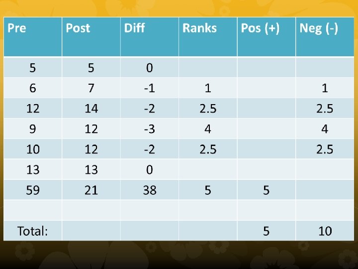
Example • Intervention: Eating a smart cookie • Academic Performance for 7 students –Pre {5, 6, 12, 9, 10, 13, 59} –Post {5, 7, 14, 12, 13, 21} • Bumble decided to use paired samples t-test. Would you accept Bumble’s analysis? Why or why not?

Issues? Fails to meet the assumptions of paired samples t-test. Non-normal distribution of difference scores Also, small sample size makes parametric test more vulnerable to effects of violations of assumptions

Wilcoxon T • Why do we use it? – Nonparametric version of the matched samples t-test – Concerned about extreme outliers messing with data • Ho: The sum of ranks of the positive difference scores = The sum of ranks of the negative difference scores • How do you use it? – Based on score ranking, and then summing scores for positive and negative differences, use smallest to get your T. – Remember to ignore difference scores of zero. – Outliers are based on difference scores, not actual scores.

Chi-Square (χ2) • Why? – Tests whether the data that we observe (frequencies) differ from our expectation based on a model such as independent of two variables. • When? – fe>5 → χ2 test • H 0: independence between the row and column variables in the population • How? – χ2 =∑(fo-fe)2/fe – df=(#rows-1)*(#columns-1) – Critical χ2 =3. 84 when 2 x 2 • Yates correction for continuity – χ2 =∑(|fo-fe|-0. 5)2/fe – when df=1 and margins are fixed before collecting data

Fisher’s exact Test • When? – fe<5 – If fe is small, it may distort a χ2 value (check the denominator of formula!) • How? – Prob=(a+b)!(c+d)!(a+c)!(b+d)! N!a!b!c!d! – Probability of the exact outcome, sum with more extreme outcomes

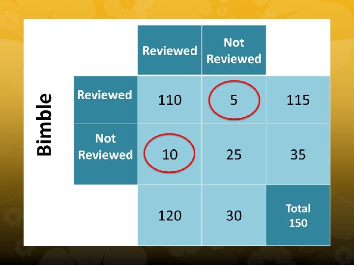
Example Bumble and Bimble were auditors for the IRS. One task was to review tax returns to determine whether the return should be audited. Bumble and Bimble each reviewed the sample of 150 returns. Bumble selected 120 that should be reviewed and Bimble selected 115 to be reviewed, but there were only 110 returns they both reviewed. Do they differ significantly in their selection rates?

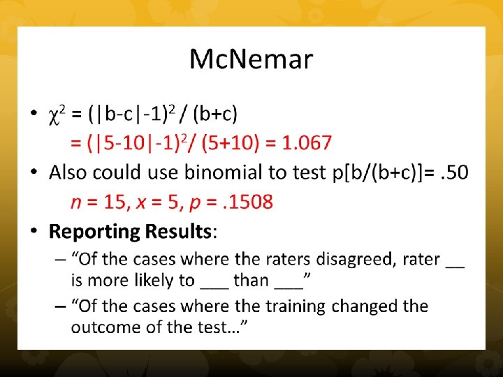
+ - a b a+b c d c+d a+c b+d Mc. Nemar N • Why? – To tests the likelihood of an event: • Is Rater 1 more likely to say + (or -) than Rater 2? • Do more people Pass (or Fail) test after training? • Null hypothesis – H 0: p(+| X)=p(+| Y), (a+b)/N=(a+c)/N; Are marginal distributions same? – H 0 can be boiled down to… b=c ∴ Mc. Nemar uses disagreement cells to answer these questions! • How? (1) χ2 approximation • χ2 = (|b-c|-1)2/(b+c) if Npq>5, Always df=1, critical χ2 . 05=3. 84 • N is not total N, but total of two cell (b+c) (2) Binomial test (p. 34 Siegel’s Table D)

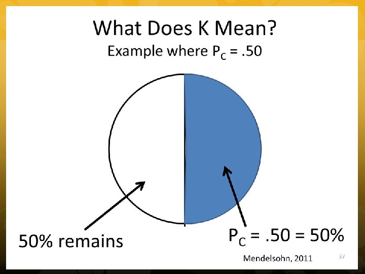
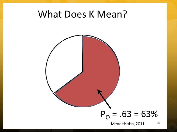
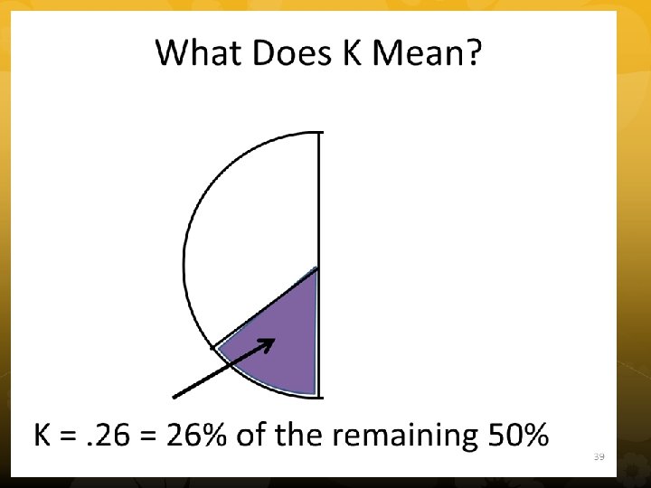
Cohen’s Kappa • To test extent of agreement • Percent observed (Po) and Percent chance (Pc) agreement • Test significance with chi square

Example • People are waiting in line at the Apple store to purchase the i. Phone 5. Its an exclusive offer and its 3 am, but people are already there! • MMMFFFFMMMMMFFF • Are people of the same gender lining up in clusters more than we would expect by chance?

Runs test • Why? – Test for Serial Randomness of Nominal Data – Q: Is the order of two mixed groups more (or less) scrambled than would be expected by chance? • H 0: random dispersion of nominal data • How? – Use Siegel’s table F 1&2 (p. 38) – If R < the lower RCritical (“too few” table) then the data are nonrandom due to clustering. – If R > the upper RCritical (“too many” table) then the data are nonrandom due to uniformity. – If R falls between the lower and upper RCritical then the data are consistent with random mixing of cases.

Runs • In our example, bigger clusters = less runs • Are there too few runs? • MMM, FFFF, MMMMM, FFF • N 1 = 7, N 2= 8, R = 4 • Siegel (1956) table on p. 36, p <. 05 • Value shown on table or smaller is sig.

Happy Studying! • Read Question carefully – create a table with the numbers – think about which test is most appropriate • Recall some of the basics – Assumptions – Null hypotheses – P-values