Classification 1 l Classification predict categorical class labels

Classification 1

分類與預測 l Classification (分類) Øpredict categorical class labels 預測分門別類的類別 標籤 ncategorical class labels: 離散式的或名目式的 (discrete/nominal) Ø根據訓練組資料的分類屬性的值（即類別標籤）， 建構一個模型，並以之將新資料歸類 l Prediction (預測) Ømodel continuous-valued functions 掌握連續值型態 的函數，預測未知或遺失的值 2 Ming-Yen Lin, IECS, FCU

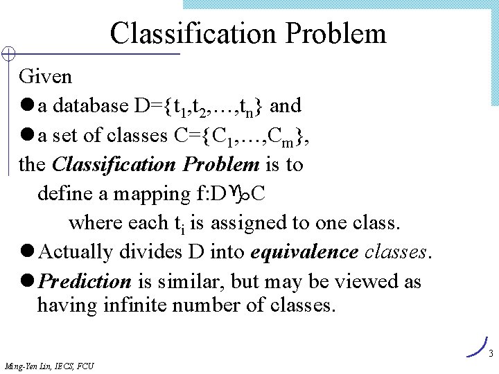
Classification Problem Given l a database D={t 1, t 2, …, tn} and l a set of classes C={C 1, …, Cm}, the Classification Problem is to define a mapping f: Dg. C where each ti is assigned to one class. l Actually divides D into equivalence classes. l Prediction is similar, but may be viewed as having infinite number of classes. 3 Ming-Yen Lin, IECS, FCU

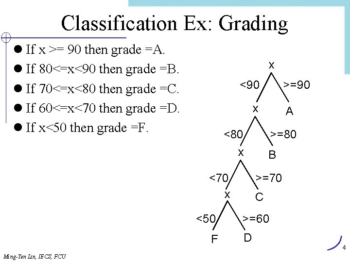
Classification Ex: Grading l If x >= 90 then grade =A. l If 80<=x<90 then grade =B. l If 70<=x<80 then grade =C. l If 60<=x<70 then grade =D. l If x<50 then grade =F. x <90 x <80 x <70 x <50 F Ming-Yen Lin, IECS, FCU >=90 A >=80 B >=70 C >=60 D 4

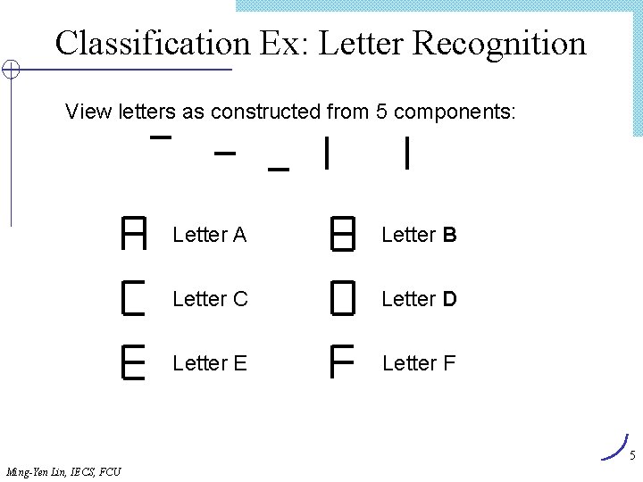
Classification Ex: Letter Recognition View letters as constructed from 5 components: Letter A Letter B Letter C Letter D Letter E Letter F 5 Ming-Yen Lin, IECS, FCU

Classification Examples l Teachers classify students’ grades as A, B, C, D, or F. l Identify mushrooms as poisonous or edible. l Classify a river as flooding or not. l Identify an individual as certain credit risk. l Speech recognition: Identify the spoken “word” from the classified examples (rules). l Pattern recognition: Identify a pattern from the classified ones. l 典型應用 Ø 信用核發，目標行銷，醫療診斷，處方(treatment)有效性 分析 6 Ming-Yen Lin, IECS, FCU

Classification—兩大步驟 l 建構模型: 描述一組預定的類別（predetermined class） Ø 每筆資料皆已具有預定的類別（由 class label attribute決定） Ø training set : 用來建構模型的資料組 Ø 模型的呈現：(1) classification rules (2) decision trees (3) mathematical formulae l 使用模型: 將未來或未知之objects分類 Ø 估計模型之 accuracy n 將已知類別的test sample灌入模型，比較模型的答案類別 n Accuracy rate： test set samples正確被模型分類的比例 n Test set：獨立於 training set, 否則會over-fitting Ø 若accuracy 可接受，用此模型將未知類別標籤的資料項分類 l Most common techniques use DTs, NNs, or are based on distances or statistical methods 7 Ming-Yen Lin, IECS, FCU

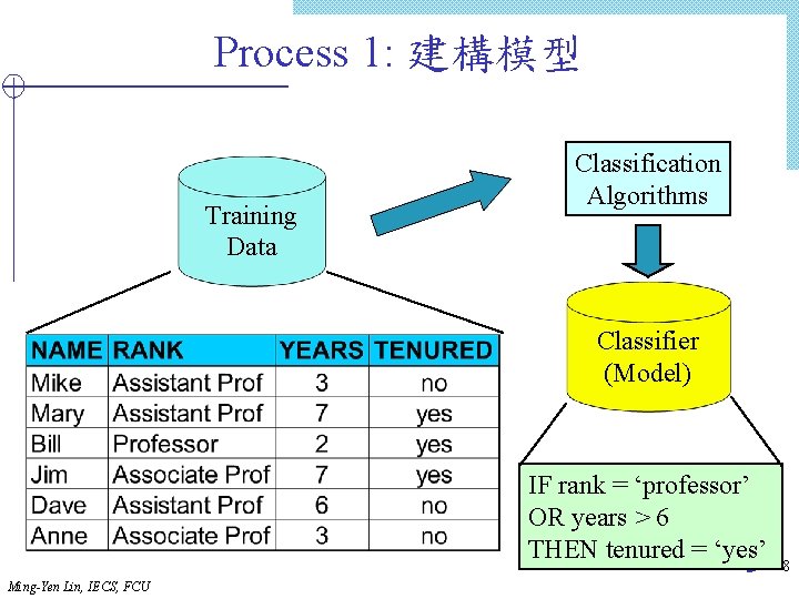
Process 1: 建構模型 Training Data Classification Algorithms Classifier (Model) IF rank = ‘professor’ OR years > 6 THEN tenured = ‘yes’ Ming-Yen Lin, IECS, FCU 8

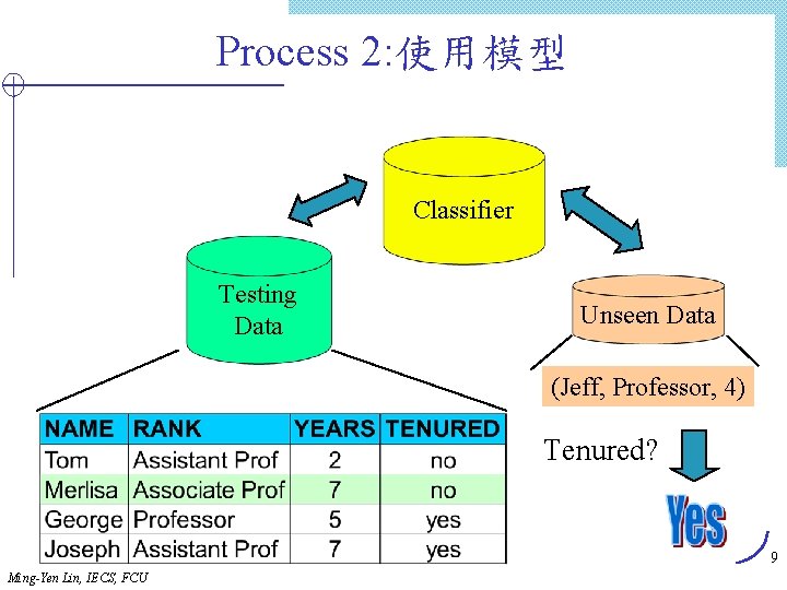
Process 2: 使用模型 Classifier Testing Data Unseen Data (Jeff, Professor, 4) Tenured? 9 Ming-Yen Lin, IECS, FCU

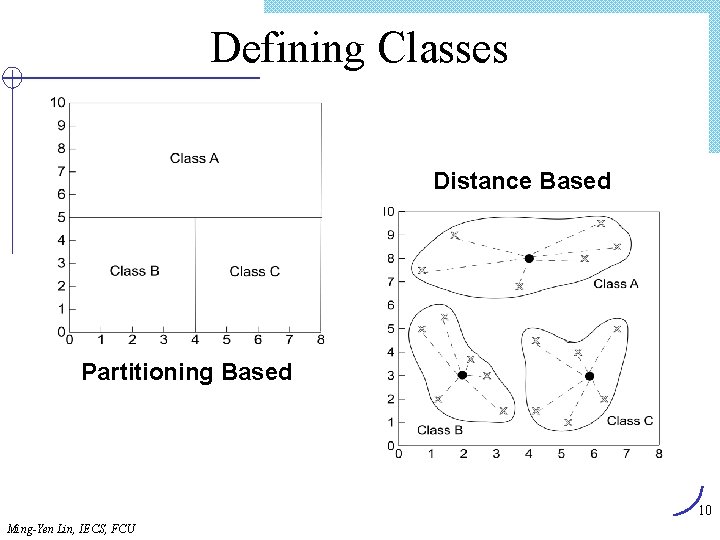
Defining Classes Distance Based Partitioning Based 10 Ming-Yen Lin, IECS, FCU

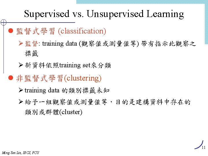
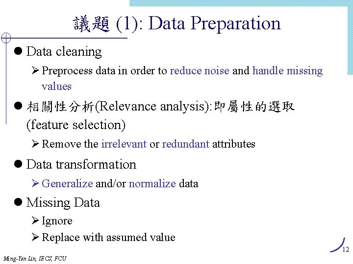
議題 (1): Data Preparation l Data cleaning Ø Preprocess data in order to reduce noise and handle missing values l 相關性分析(Relevance analysis): 即屬性的選取 (feature selection) Ø Remove the irrelevant or redundant attributes l Data transformation Ø Generalize and/or normalize data l Missing Data Ø Ignore Ø Replace with assumed value 12 Ming-Yen Lin, IECS, FCU

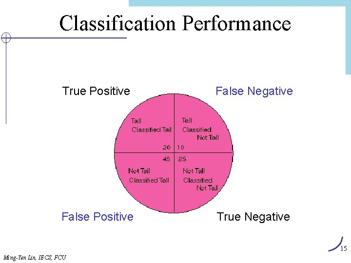
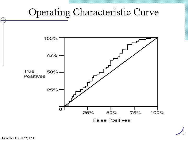
議題(2): 評估 Classification Methods l 預測準確率(Predictive accuracy) Ø Classification accuracy on test data Ø Confusion matrix Ø OC Curve l 速度與可擴充性( scalability) Ø 建構 classifier 的時間多久 Ø 何時可以使用classifier l 強固性(Robustness) Ø handling noise and missing values l 可擴充性(Scalability) Ø disk-resident databases 的效率 l 可解釋性(Interpretability) Ø 對model的瞭解與model可提供的insight(瞭解深度) l rule有多好（ goodness measure ） Ø decision tree size Ø compactness of classification rules 13 Ming-Yen Lin, IECS, FCU

Height Example Data accuracy 14 Ming-Yen Lin, IECS, FCU

Classification Performance True Positive False Negative False Positive True Negative 15 Ming-Yen Lin, IECS, FCU

Confusion Matrix Example Using height data example with Output 1 correct and Output 2 actual assignment 16 Ming-Yen Lin, IECS, FCU

Operating Characteristic Curve 17 Ming-Yen Lin, IECS, FCU

Classification Using Decision Trees l Partitioning based: Divide search space into rectangular regions. l Tuple placed into class based on the region within which it falls. l DT approaches differ in how the tree is built: DT Induction l Internal nodes associated with attribute and arcs with values for that attribute. l Algorithms: ID 3, C 4. 5, CART 18 Ming-Yen Lin, IECS, FCU

Decision Tree Given: ØD = {t 1, …, tn} where ti=<ti 1, …, tih> ØDatabase schema contains {A 1, A 2, …, Ah} ØClasses C={C 1, …. , Cm} Decision or Classification Tree is a tree associated with D such that ØEach internal node is labeled with attribute, Ai ØEach arc is labeled with predicate which can be applied to attribute at parent ØEach leaf node is labeled with a class, Cj 19 Ming-Yen Lin, IECS, FCU

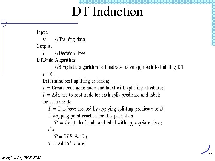
DT Induction 20 Ming-Yen Lin, IECS, FCU

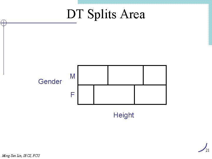
DT Splits Area Gender M F Height 21 Ming-Yen Lin, IECS, FCU

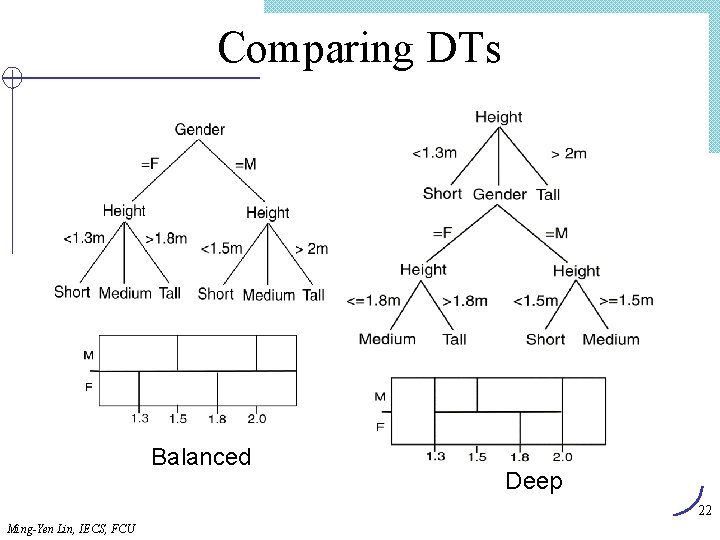
Comparing DTs Balanced Deep 22 Ming-Yen Lin, IECS, FCU

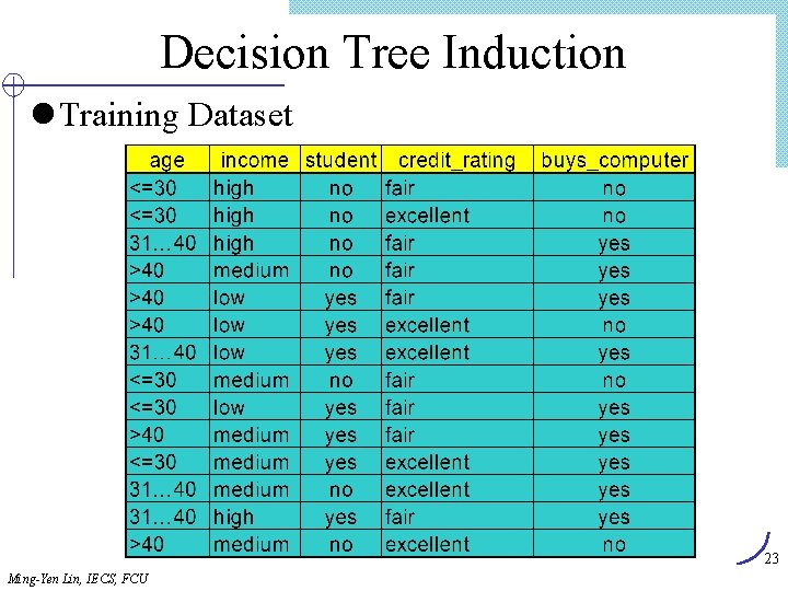
Decision Tree Induction l Training Dataset 23 Ming-Yen Lin, IECS, FCU

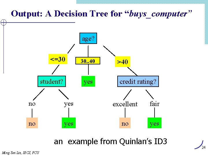
Output: A Decision Tree for “buys_computer” age? <=30 student? overcast 30. . 40 yes >40 credit rating? no yes excellent fair no yes an example from Quinlan’s ID 3 Ming-Yen Lin, IECS, FCU 24

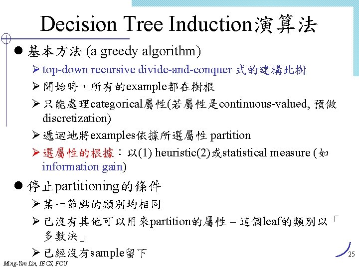
Decision Tree Induction演算法 l 基本方法 (a greedy algorithm) Ø top-down recursive divide-and-conquer 式的建構此樹 Ø 開始時，所有的example都在樹根 Ø 只能處理categorical屬性(若屬性是continuous-valued, 預做 discretization) Ø 遞迴地將examples依據所選屬性 partition Ø 選屬性的根據：以(1) heuristic(2)或statistical measure (如 information gain) l 停止partitioning的條件 Ø 某一節點的類別均相同 Ø 已沒有其他可以用來partition的屬性 – 這個leaf的類別以「 多數決」 Ø 已經沒有sample留下 Ming-Yen Lin, IECS, FCU 25

Decision Tree Induction is often based on Information Theory So 26 Ming-Yen Lin, IECS, FCU

Information 27 Ming-Yen Lin, IECS, FCU

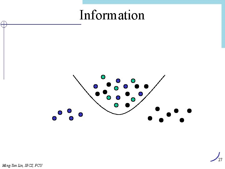
DT Induction l When all the marbles in the bowl are mixed up, little information is given. l When the marbles in the bowl are all from one class and those in the other two classes are on either side, more information is given. Use this approach with DT Induction ! 28 Ming-Yen Lin, IECS, FCU

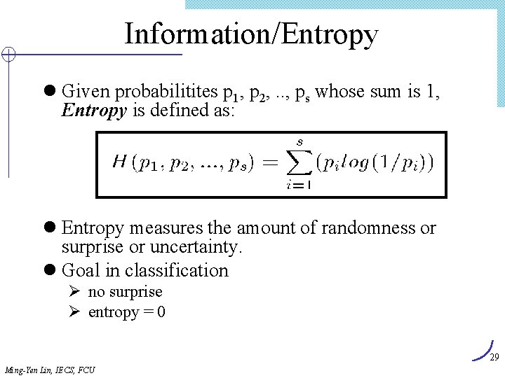
Information/Entropy l Given probabilitites p 1, p 2, . . , ps whose sum is 1, Entropy is defined as: l Entropy measures the amount of randomness or surprise or uncertainty. l Goal in classification Ø no surprise Ø entropy = 0 29 Ming-Yen Lin, IECS, FCU

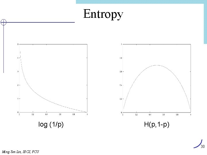
Entropy log (1/p) H(p, 1 -p) 30 Ming-Yen Lin, IECS, FCU

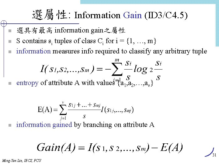
選屬性: Information Gain (ID 3/C 4. 5) n 選具有最高 information gain之屬性 S contains si tuples of class Ci for i = {1, …, m} information measures info required to classify any arbitrary tuple n entropy of attribute A with values {a 1, a 2, …, av} n information gained by branching on attribute A n n 31 Ming-Yen Lin, IECS, FCU

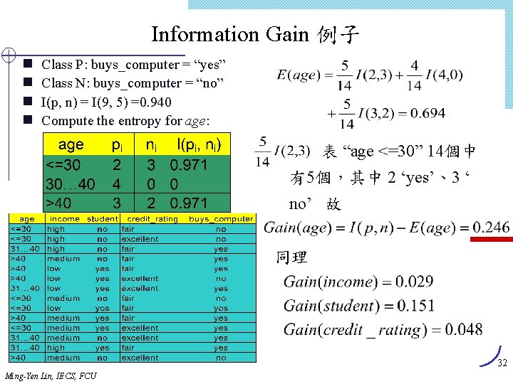
Information Gain 例子 Class P: buys_computer = “yes” g Class N: buys_computer = “no” g I(p, n) = I(9, 5) =0. 940 g Compute the entropy for age: g 表 “age <=30” 14個中 有5個，其中 2 ‘yes’、3 ‘ no’ 故 同理 32 Ming-Yen Lin, IECS, FCU

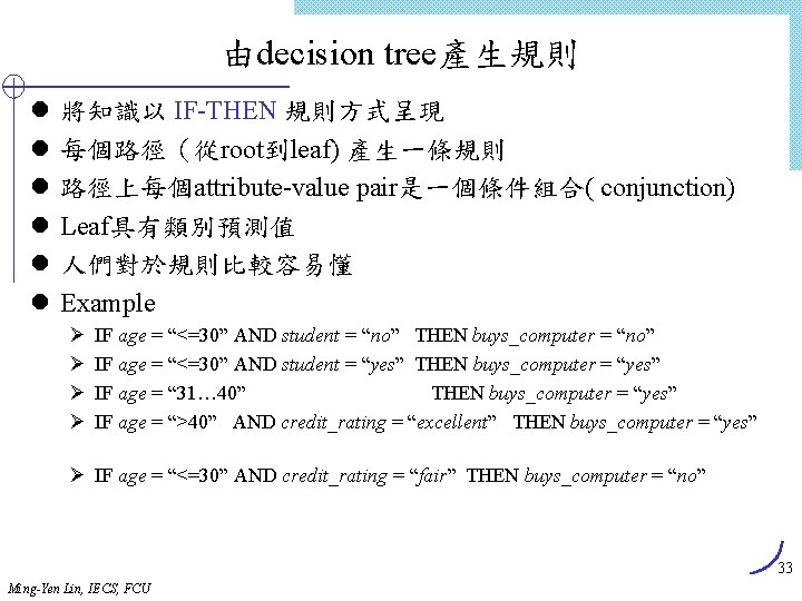
由decision tree產生規則 l l l 將知識以 IF-THEN 規則方式呈現 每個路徑（從root到leaf) 產生一條規則 路徑上每個attribute-value pair是一個條件組合( conjunction) Leaf具有類別預測值 人們對於規則比較容易懂 Example Ø Ø IF age = “<=30” AND student = “no” THEN buys_computer = “no” IF age = “<=30” AND student = “yes” THEN buys_computer = “yes” IF age = “ 31… 40” THEN buys_computer = “yes” IF age = “>40” AND credit_rating = “excellent” THEN buys_computer = “yes” Ø IF age = “<=30” AND credit_rating = “fair” THEN buys_computer = “no” 33 Ming-Yen Lin, IECS, FCU

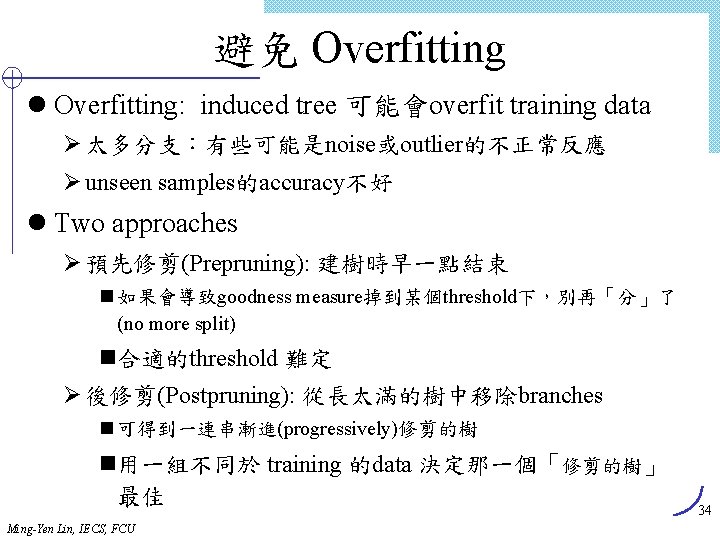
避免 Overfitting l Overfitting: induced tree 可能會overfit training data Ø 太多分支：有些可能是noise或outlier的不正常反應 Ø unseen samples的accuracy不好 l Two approaches Ø 預先修剪(Prepruning): 建樹時早一點結束 n 如果會導致goodness measure掉到某個threshold下，別再「分」了 (no more split) n合適的threshold 難定 Ø 後修剪(Postpruning): 從長太滿的樹中移除branches n 可得到一連串漸進(progressively)修剪的樹 n用一組不同於 training 的data 決定那一個「修剪的樹」 最佳 Ming-Yen Lin, IECS, FCU 34

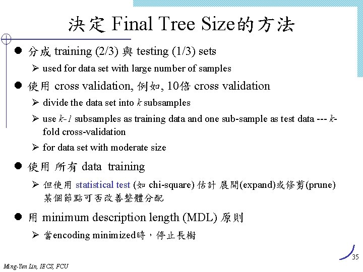
決定 Final Tree Size的方法 l 分成 training (2/3) 與 testing (1/3) sets Ø used for data set with large number of samples l 使用 cross validation, 例如, 10倍 cross validation Ø divide the data set into k subsamples Ø use k-1 subsamples as training data and one sub-sample as test data --- kfold cross-validation Ø for data set with moderate size l 使用 所有 data training Ø 但使用 statistical test (如 chi-square) 估計 展開(expand)或修剪(prune) 某個節點可否改善整體分配 l 用 minimum description length (MDL) 原則 Ø 當encoding minimized時，停止長樹 35 Ming-Yen Lin, IECS, FCU

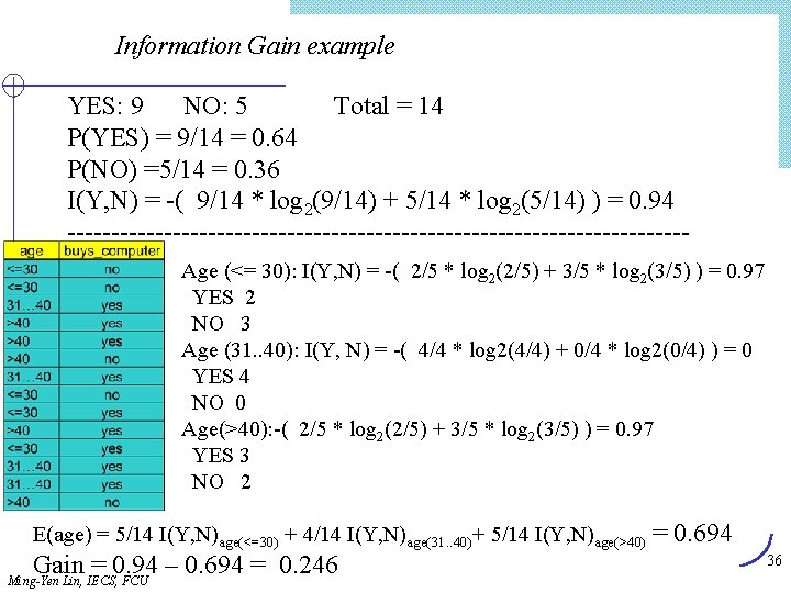
Information Gain example YES: 9 NO: 5 Total = 14 P(YES) = 9/14 = 0. 64 P(NO) =5/14 = 0. 36 I(Y, N) = -( 9/14 * log 2(9/14) + 5/14 * log 2(5/14) ) = 0. 94 -----------------------------------Age (<= 30): I(Y, N) = -( 2/5 * log 2(2/5) + 3/5 * log 2(3/5) ) = 0. 97 YES 2 NO 3 Age (31. . 40): I(Y, N) = -( 4/4 * log 2(4/4) + 0/4 * log 2(0/4) ) = 0 YES 4 NO 0 Age(>40): -( 2/5 * log 2(2/5) + 3/5 * log 2(3/5) ) = 0. 97 YES 3 NO 2 E(age) = 5/14 I(Y, N)age(<=30) + 4/14 I(Y, N)age(31. . 40)+ 5/14 I(Y, N)age(>40) = 0. 694 Gain = 0. 94 – 0. 694 = 0. 246 Ming-Yen Lin, IECS, FCU 36

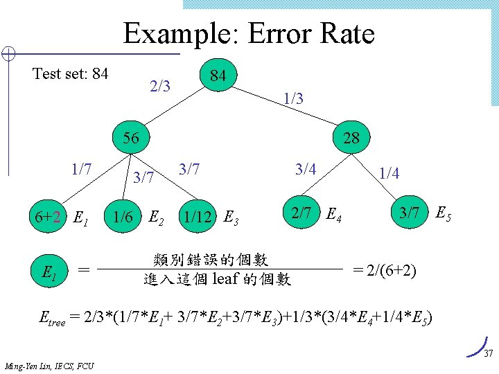
Example: Error Rate Test set: 84 84 2/3 1/3 56 1/7 6+2 E 1 ＝ 28 3/7 1/6 E 2 3/7 3/4 1/12 E 3 2/7 E 4 類別錯誤的個數 進入這個 leaf 的個數 1/4 3/7 E 5 = 2/(6+2) Etree = 2/3*(1/7*E 1+ 3/7*E 2+3/7*E 3)+1/3*(3/4*E 4+1/4*E 5) 37 Ming-Yen Lin, IECS, FCU

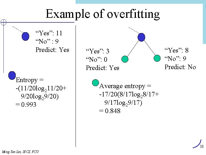
Example of overfitting “Yes”: 11 “No” : 9 Predict: Yes Entropy = -(11/20 log 211/20+ 9/20 log 29/20) = 0. 993 “Yes”: 3 “No”: 0 Predict: Yes “Yes”: 8 “No”: 9 Predict: No Average entropy = -17/20(8/17 log 28/17+ 9/17 log 29/17) = 0. 848 38 Ming-Yen Lin, IECS, FCU

強化(enhance)基本決策樹 l 允許 continuous-valued 屬性 Ø 動態定義將continuous attribute value partition為離散區間的 新離散屬性 l 處理 missing attribute values Ø 指定共通值 Ø 指定各個值的機率 l 建立Attribute Ø 為現有稀疏的屬性(sparsely represented)建立新attribute Ø 可減少(簡化) fragmentation, repetition, and replication 39 Ming-Yen Lin, IECS, FCU

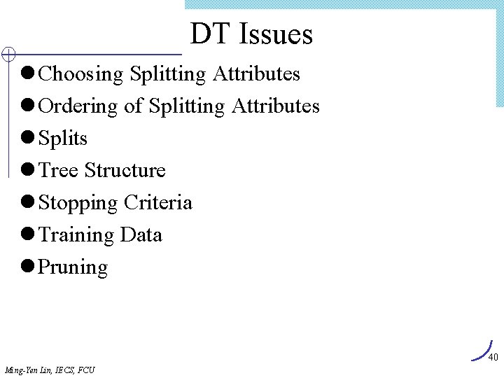
DT Issues l Choosing Splitting Attributes l Ordering of Splitting Attributes l Splits l Tree Structure l Stopping Criteria l Training Data l Pruning 40 Ming-Yen Lin, IECS, FCU

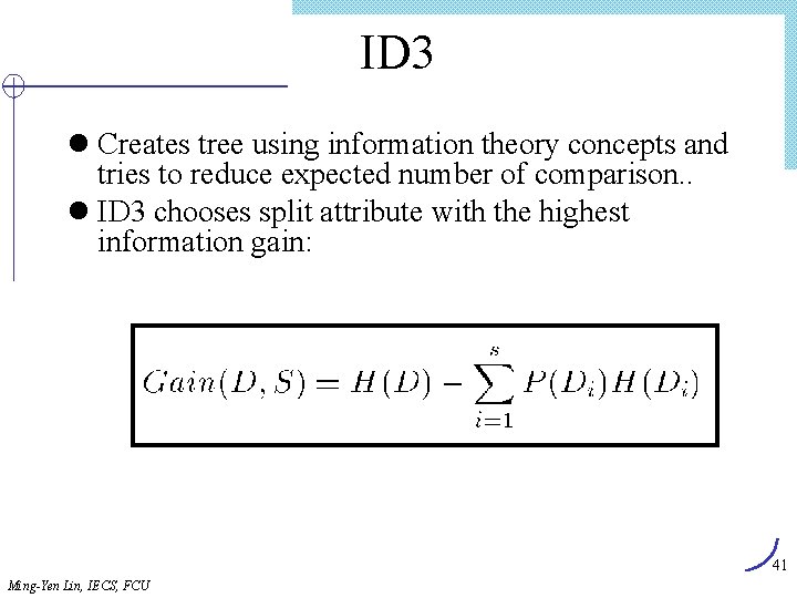
ID 3 l Creates tree using information theory concepts and tries to reduce expected number of comparison. . l ID 3 chooses split attribute with the highest information gain: 41 Ming-Yen Lin, IECS, FCU

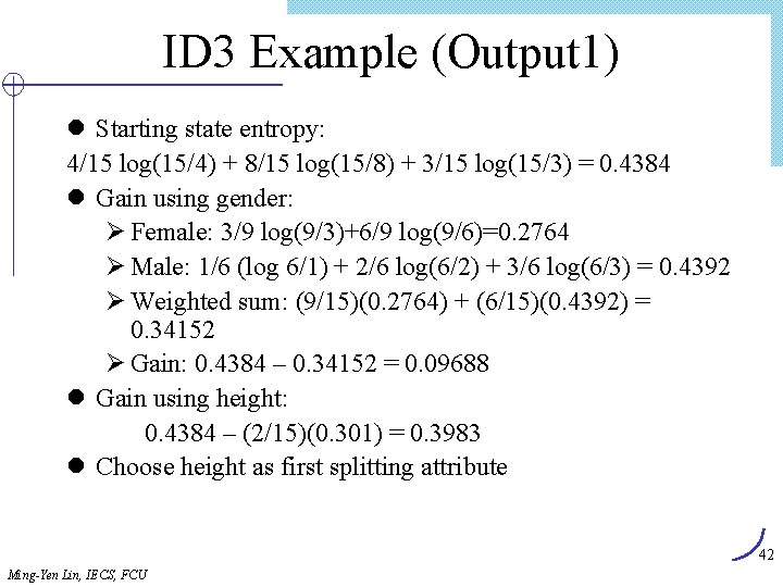
ID 3 Example (Output 1) l Starting state entropy: 4/15 log(15/4) + 8/15 log(15/8) + 3/15 log(15/3) = 0. 4384 l Gain using gender: Ø Female: 3/9 log(9/3)+6/9 log(9/6)=0. 2764 Ø Male: 1/6 (log 6/1) + 2/6 log(6/2) + 3/6 log(6/3) = 0. 4392 Ø Weighted sum: (9/15)(0. 2764) + (6/15)(0. 4392) = 0. 34152 Ø Gain: 0. 4384 – 0. 34152 = 0. 09688 l Gain using height: 0. 4384 – (2/15)(0. 301) = 0. 3983 l Choose height as first splitting attribute 42 Ming-Yen Lin, IECS, FCU

CART, C 4. 5, CHAID l Classification And Regression Tree Ømaximize diversitybefore- diversityafter ndiversity分散度-僅含單一類別之diversity低 – eg. entropy/information – compute I(2, 3, 9)? l C 4. 5 Ø Post-pruning l CHAID Ø A tree is “pruned” by halting its construction early. (Pre-pruning) Ø CHAID is restricted to categorical variables Ø Continuous variables must be broken into ranges or replaced with classes such as high, low, medium Ming-Yen Lin, IECS, FCU 43

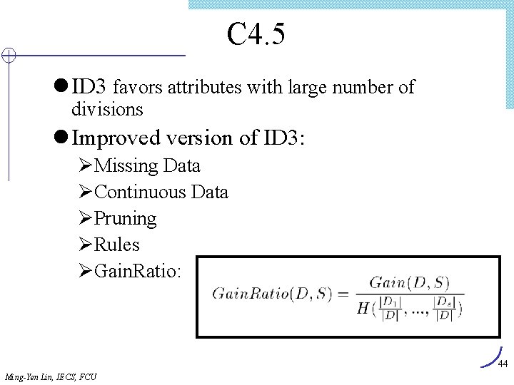
C 4. 5 l ID 3 favors attributes with large number of divisions l Improved version of ID 3: ØMissing Data ØContinuous Data ØPruning ØRules ØGain. Ratio: 44 Ming-Yen Lin, IECS, FCU

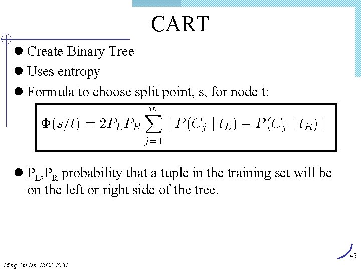
CART l Create Binary Tree l Uses entropy l Formula to choose split point, s, for node t: l PL, PR probability that a tuple in the training set will be on the left or right side of the tree. 45 Ming-Yen Lin, IECS, FCU

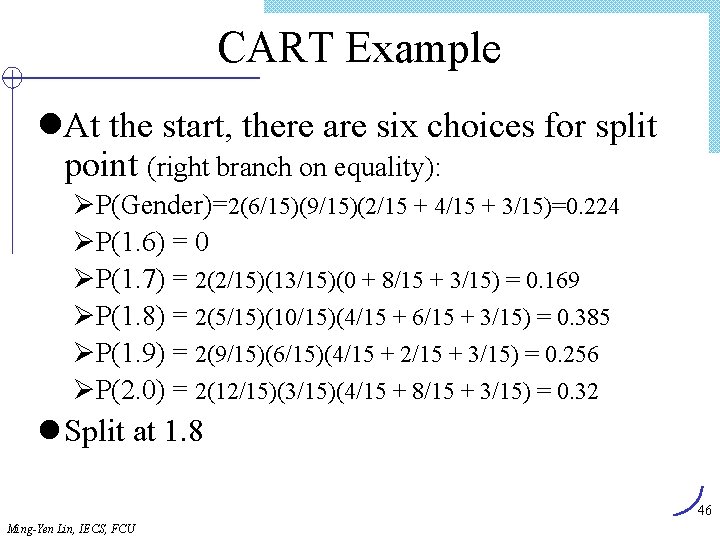
CART Example l. At the start, there are six choices for split point (right branch on equality): ØP(Gender)=2(6/15)(9/15)(2/15 + 4/15 + 3/15)=0. 224 ØP(1. 6) = 0 ØP(1. 7) = 2(2/15)(13/15)(0 + 8/15 + 3/15) = 0. 169 ØP(1. 8) = 2(5/15)(10/15)(4/15 + 6/15 + 3/15) = 0. 385 ØP(1. 9) = 2(9/15)(6/15)(4/15 + 2/15 + 3/15) = 0. 256 ØP(2. 0) = 2(12/15)(3/15)(4/15 + 8/15 + 3/15) = 0. 32 l Split at 1. 8 46 Ming-Yen Lin, IECS, FCU

Classification in Large Databases l Classification—a classical problem extensively studied by statisticians and machine learning researchers l Scalability: Classifying data sets with millions of examples and hundreds of attributes with reasonable speed l Why decision tree induction in data mining? Ø relatively faster learning speed (than other classification methods) Ø convertible to simple and easy to understand classification rules Ø can use SQL queries for accessing databases Ø comparable classification accuracy with other methods Ming-Yen Lin, IECS, FCU 47

Scalable Decision Tree Induction in Data Mining l SLIQ (EDBT’ 96 — Mehta et al. ) Ø builds an index for each attribute and only class list and the current attribute list reside in memory l SPRINT (VLDB’ 96 — J. Shafer et al. ) Ø constructs an attribute list data structure l PUBLIC (VLDB’ 98 — Rastogi & Shim) Ø integrates tree splitting and tree pruning: stop growing the tree earlier l Rain. Forest (VLDB’ 98 — Gehrke, Ramakrishnan & Ganti) Ø separates the scalability aspects from the criteria that determine the quality of the tree Ø builds an AVC-list (attribute, value, class label) Ming-Yen Lin, IECS, FCU 48

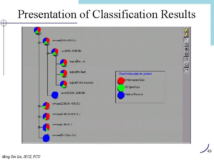
Presentation of Classification Results 49 Ming-Yen Lin, IECS, FCU

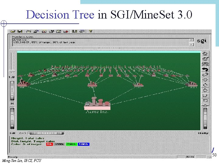
Decision Tree in SGI/Mine. Set 3. 0 50 Ming-Yen Lin, IECS, FCU

Tool: Decision Tree l C 4. 5, the “classic” decision-tree tool, developed by J. Q. Quinlan Øhttp: //www. cse. unsw. edu. tw/~quinlan l Classification Tree in Excel l EC 4. 5, a more efficient version of C 4. 5 Øhttp: //www. -kdd. di. unipi. it/software l IND, provides Gini and C 4. 5 decision trees Øhttp: //ic. arc. nasa. gov/projects/bayes-group/ind/INDprogram. html 51 Ming-Yen Lin, IECS, FCU

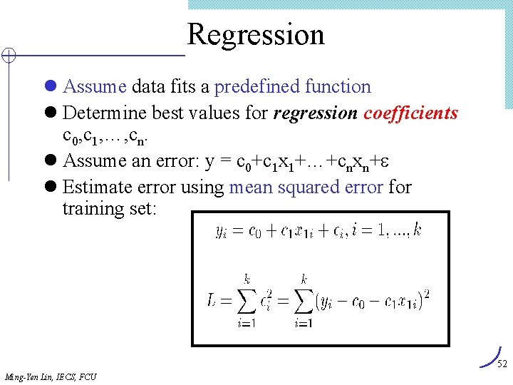
Regression l Assume data fits a predefined function l Determine best values for regression coefficients c 0, c 1, …, cn. l Assume an error: y = c 0+c 1 x 1+…+cnxn+e l Estimate error using mean squared error for training set: 52 Ming-Yen Lin, IECS, FCU

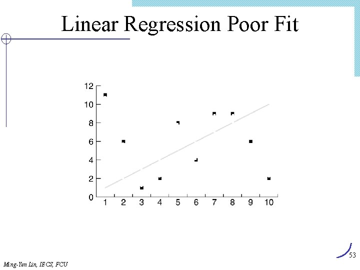
Linear Regression Poor Fit 53 Ming-Yen Lin, IECS, FCU

Classification Using Regression l Division: Use regression function to divide area into regions. l Prediction: Use regression function to predict a class membership function. Input includes desired class. 54 Ming-Yen Lin, IECS, FCU

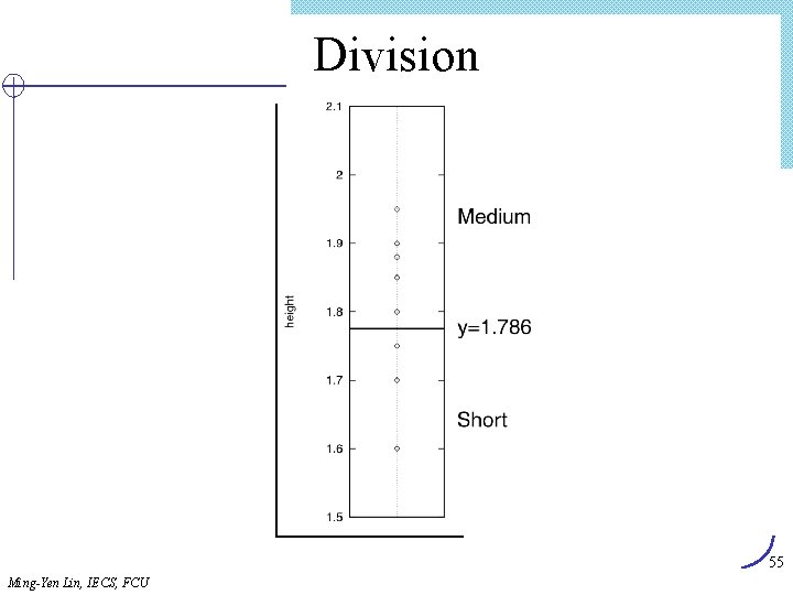
Division 55 Ming-Yen Lin, IECS, FCU

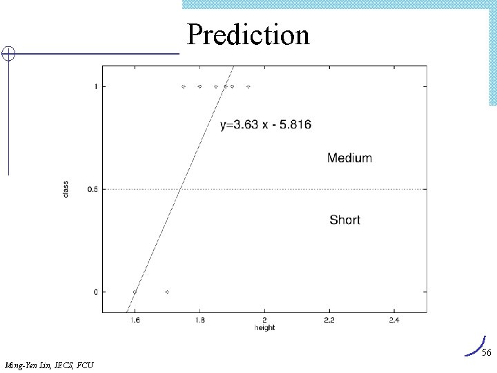
Prediction 56 Ming-Yen Lin, IECS, FCU

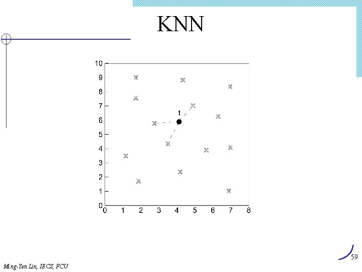
Classification Using Distance l Place items in class to which they are “closest”. l Must determine distance between an item and a class. l Classes represented by ØCentroid: Central value. ØMedoid: Representative point. ØIndividual points l. Algorithm: KNN 57 Ming-Yen Lin, IECS, FCU

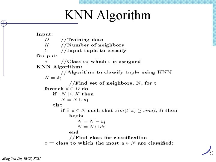
K Nearest Neighbor (KNN): l Training set includes classes. l Examine K items near item to be classified. l New item placed in class with the most number of close items. l O(q) for each tuple to be classified. (Here q is the size of the training set. ) 58 Ming-Yen Lin, IECS, FCU

KNN 59 Ming-Yen Lin, IECS, FCU

KNN Algorithm 60 Ming-Yen Lin, IECS, FCU

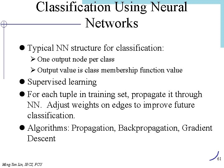
Classification Using Neural Networks l Typical NN structure for classification: Ø One output node per class Ø Output value is class membership function value l Supervised learning l For each tuple in training set, propagate it through NN. Adjust weights on edges to improve future classification. l Algorithms: Propagation, Backpropagation, Gradient Descent 61 Ming-Yen Lin, IECS, FCU

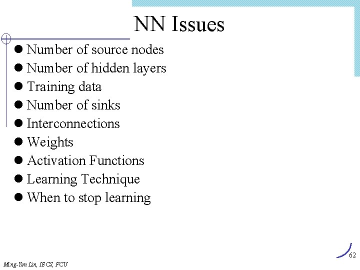
NN Issues l Number of source nodes l Number of hidden layers l Training data l Number of sinks l Interconnections l Weights l Activation Functions l Learning Technique l When to stop learning 62 Ming-Yen Lin, IECS, FCU

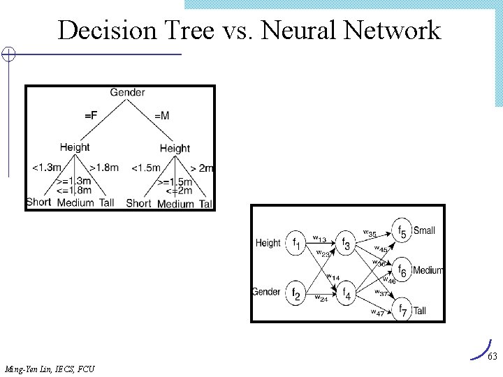
Decision Tree vs. Neural Network 63 Ming-Yen Lin, IECS, FCU

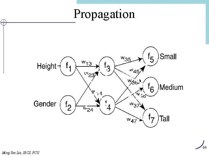
Propagation Tuple Input 64 Ming-Yen Lin, IECS, FCU

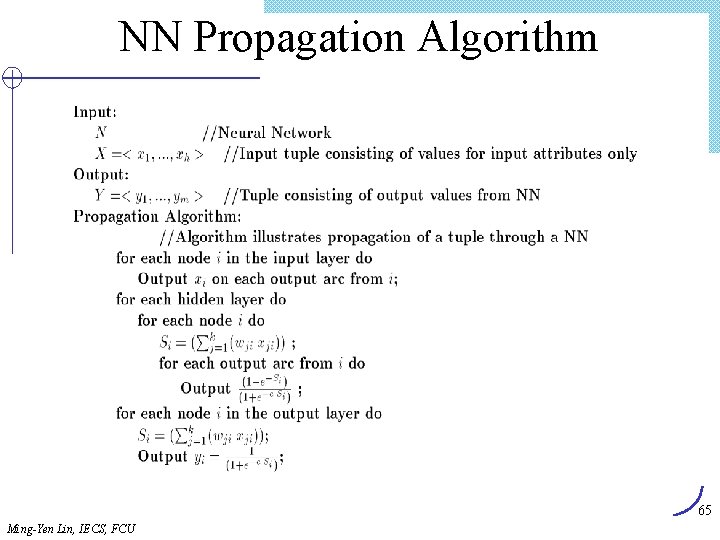
NN Propagation Algorithm 65 Ming-Yen Lin, IECS, FCU

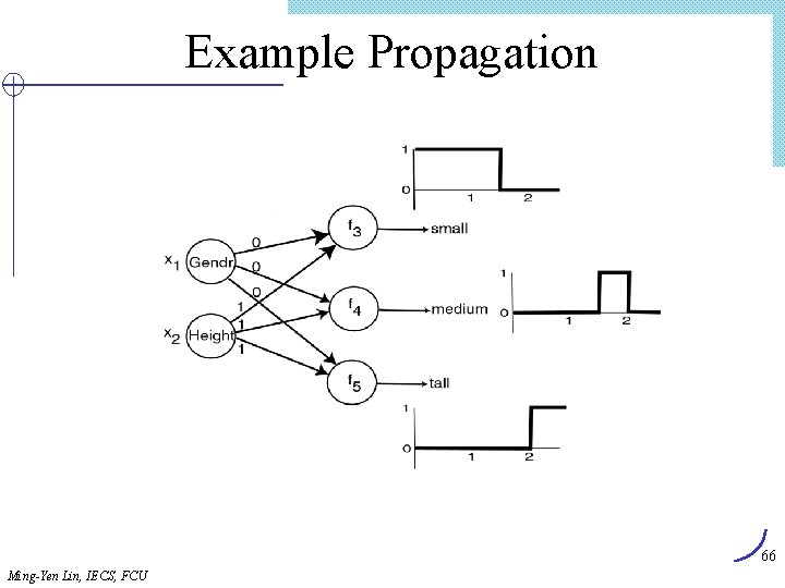
Example Propagation 66 Ming-Yen Lin, IECS, FCU

NN Learning l Adjust weights to perform better with the associated test data. l Supervised: Use feedback from knowledge of correct classification. l Unsupervised: No knowledge of correct classification needed. 67 Ming-Yen Lin, IECS, FCU

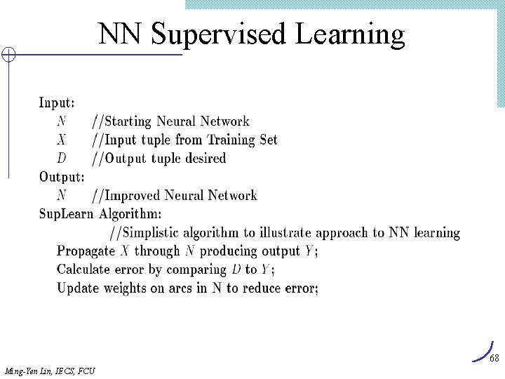
NN Supervised Learning 68 Ming-Yen Lin, IECS, FCU

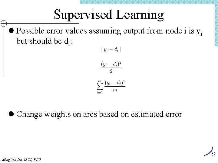
Supervised Learning l Possible error values assuming output from node i is yi but should be di: l Change weights on arcs based on estimated error 69 Ming-Yen Lin, IECS, FCU

NN Backpropagation l Propagate changes to weights backward from output layer to input layer. l Delta Rule: r wij= c xij (dj – yj) l Gradient Descent: technique to modify the weights in the graph. 70 Ming-Yen Lin, IECS, FCU

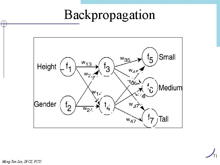
Backpropagation 71 Ming-Yen Lin, IECS, FCU

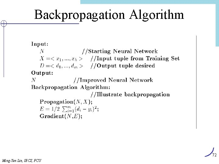
Backpropagation Algorithm 72 Ming-Yen Lin, IECS, FCU

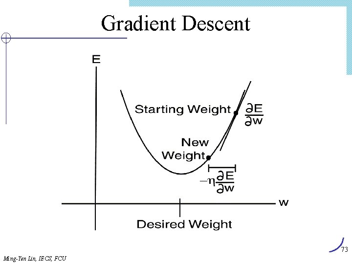
Gradient Descent 73 Ming-Yen Lin, IECS, FCU

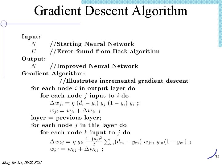
Gradient Descent Algorithm 74 Ming-Yen Lin, IECS, FCU

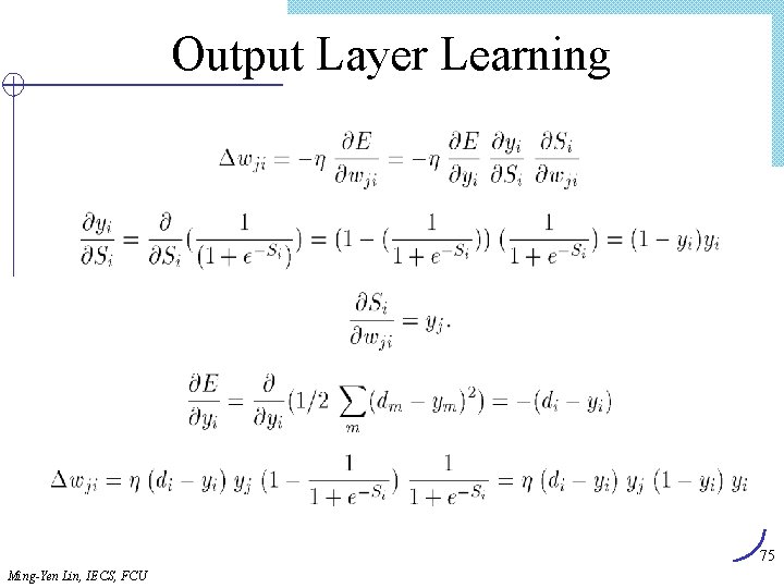
Output Layer Learning 75 Ming-Yen Lin, IECS, FCU

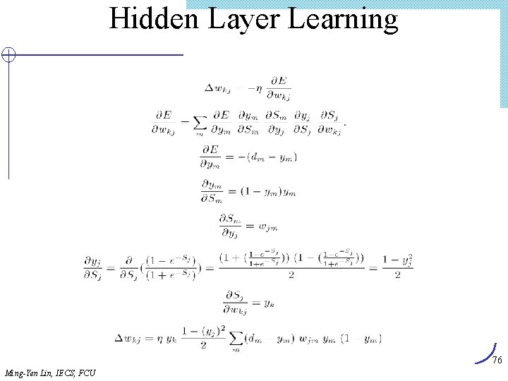
Hidden Layer Learning 76 Ming-Yen Lin, IECS, FCU

Types of NNs l Different NN structures used for different problems. l Perceptron l Self Organizing Feature Map l Radial Basis Function Network 77 Ming-Yen Lin, IECS, FCU

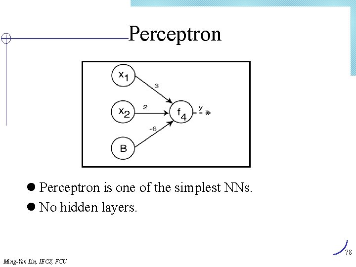
Perceptron l Perceptron is one of the simplest NNs. l No hidden layers. 78 Ming-Yen Lin, IECS, FCU

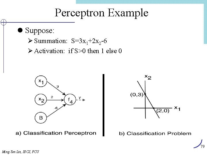
Perceptron Example l Suppose: Ø Summation: S=3 x 1+2 x 2 -6 Ø Activation: if S>0 then 1 else 0 79 Ming-Yen Lin, IECS, FCU

Self Organizing Feature Map (SOFM) l SOM l Competitive Unsupervised Learning l Observe how neurons work in brain: ØFiring impacts firing of those near ØNeurons far apart inhibit each other ØNeurons have specific nonoverlapping tasks l Ex: Kohonen Network 80 Ming-Yen Lin, IECS, FCU

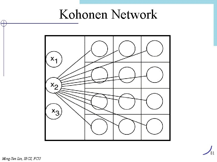
Kohonen Network 81 Ming-Yen Lin, IECS, FCU

Kohonen Network l Competitive Layer – viewed as 2 D grid l Similarity between competitive nodes and input nodes: Ø Input: X = <x 1, …, xh> Ø Weights: <w 1 i, … , whi> Ø Similarity defined based on dot product l Competitive node most similar to input “wins” l Winning node weights (as well as surrounding node weights) increased. 82 Ming-Yen Lin, IECS, FCU

Radial Basis Function Network l RBF function has Gaussian shape l RBF Networks ØThree Layers ØHidden layer – Gaussian activation function ØOutput layer – Linear activation function 83 Ming-Yen Lin, IECS, FCU

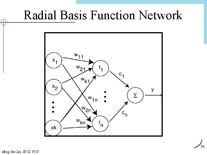
Radial Basis Function Network 84 Ming-Yen Lin, IECS, FCU

Classification Using Rules l Perform classification using If-Then rules l Classification Rule: r = <a, c> Antecedent, Consequent l May generate from other techniques (DT, NN) or generate directly. l Algorithms: Gen, RX, 1 R, PRISM 85 Ming-Yen Lin, IECS, FCU

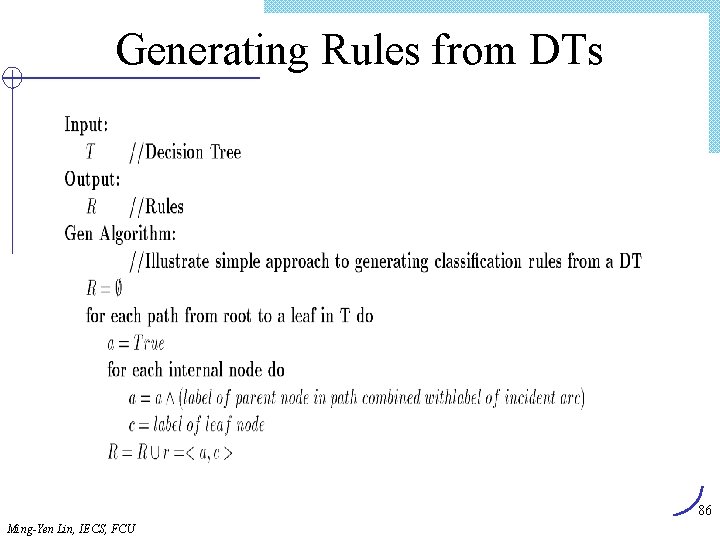
Generating Rules from DTs 86 Ming-Yen Lin, IECS, FCU

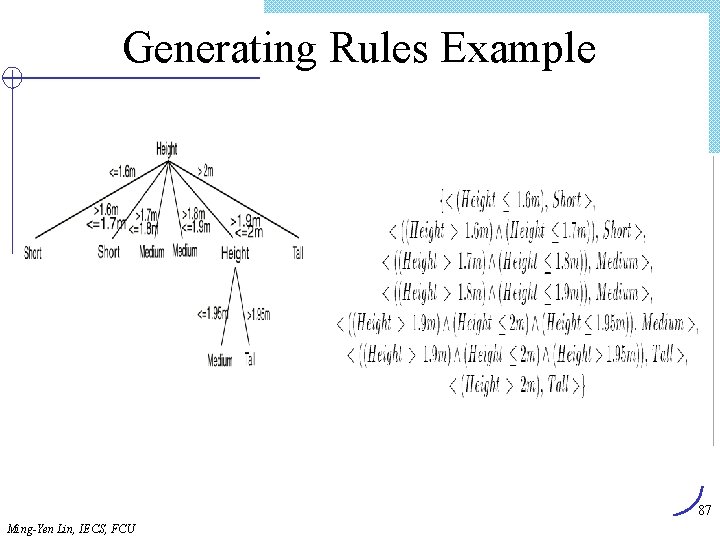
Generating Rules Example 87 Ming-Yen Lin, IECS, FCU

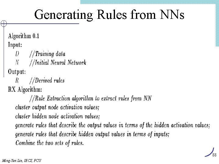
Generating Rules from NNs 88 Ming-Yen Lin, IECS, FCU

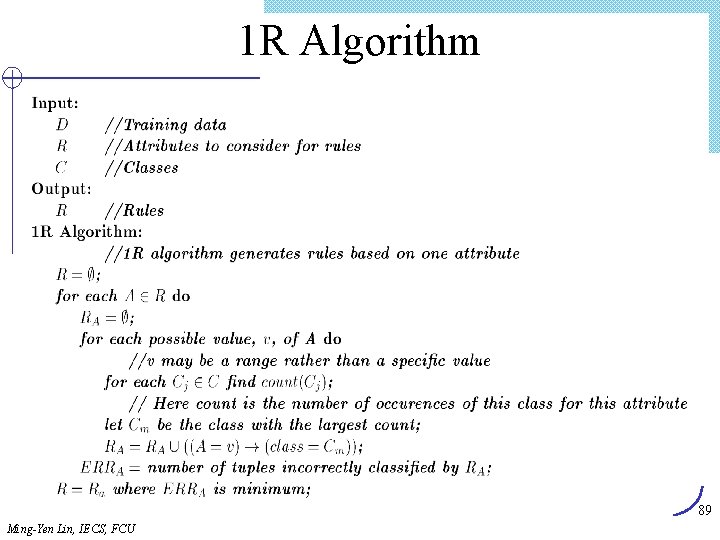
1 R Algorithm 89 Ming-Yen Lin, IECS, FCU

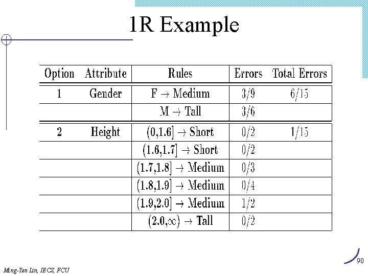
1 R Example 90 Ming-Yen Lin, IECS, FCU

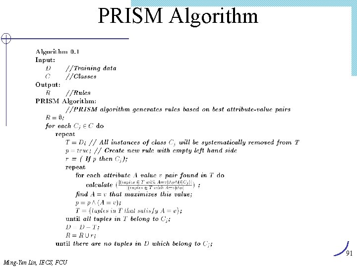
PRISM Algorithm 91 Ming-Yen Lin, IECS, FCU

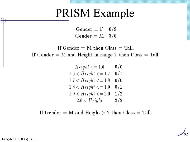
PRISM Example 92 Ming-Yen Lin, IECS, FCU

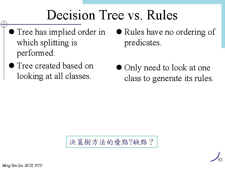
Decision Tree vs. Rules l Tree has implied order in which splitting is performed. l Tree created based on looking at all classes. l Rules have no ordering of predicates. l Only need to look at one class to generate its rules. 決策樹方法的優點? 缺點？ 93 Ming-Yen Lin, IECS, FCU