Case Control package Martijn Schuemie Marc Suchard David

- Slides: 40

Case. Control package Martijn Schuemie, Marc Suchard, David Madigan

Quick recap of previous meeting • We discussed the question ‘what question to answer? ’ – Clinicals decide on most important question – Let data decide • • • Prevalent disease Multiple prevalent treatments Outcomes that occur frequently after initiation of the treatment 2

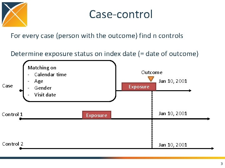
Case-control For every case (person with the outcome) find n controls Determine exposure status on index date (= date of outcome) Case Control 1 Control 2 Matching on - Calendar time - Age - Gender - Visit date Outcome Exposure Jan 10, 2001 3

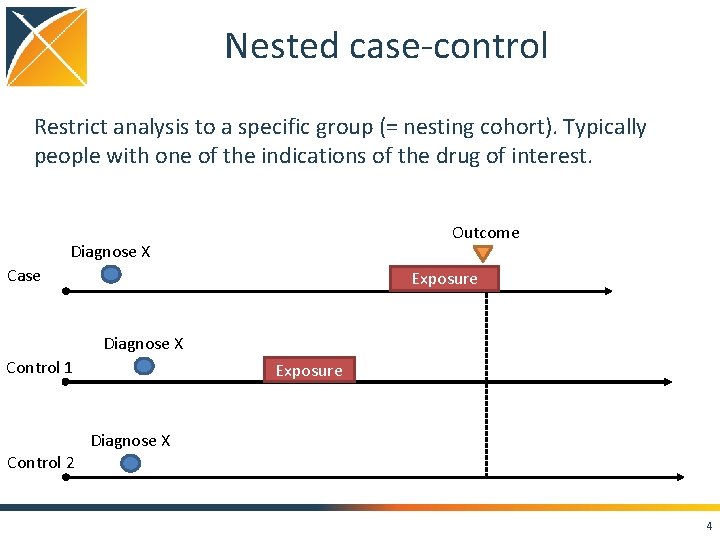
Nested case-control Restrict analysis to a specific group (= nesting cohort). Typically people with one of the indications of the drug of interest. Outcome Diagnose X Case Exposure Diagnose X Control 1 Control 2 Exposure Diagnose X 4

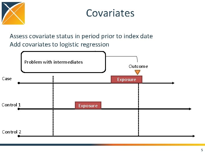
Covariates Assess covariate status in period prior to index date Add covariates to logistic regression Problem with intermediates Case Control 1 Outcome Exposure Control 2 5

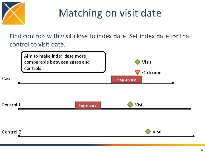
Matching on visit date Find controls with visit close to index date. Set index date for that control to visit date. Aim to make index date more comparable between cases and controls Case Control 1 Control 2 Visit Outcome Exposure Visit 6

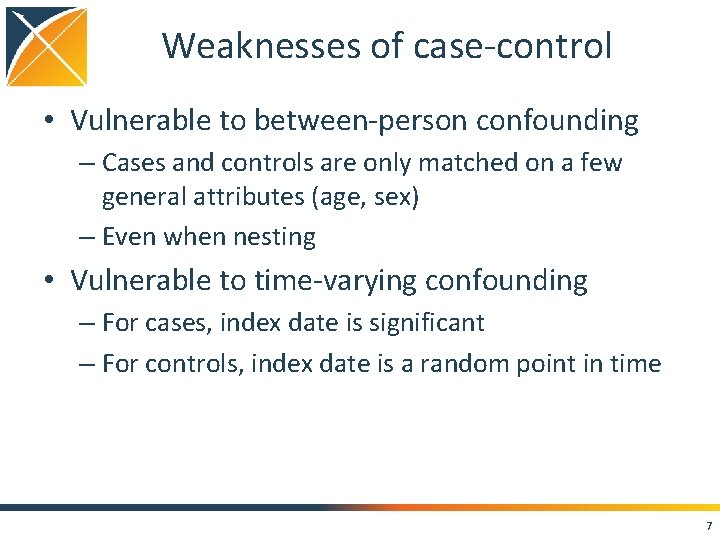
Weaknesses of case-control • Vulnerable to between-person confounding – Cases and controls are only matched on a few general attributes (age, sex) – Even when nesting • Vulnerable to time-varying confounding – For cases, index date is significant – For controls, index date is a random point in time 7

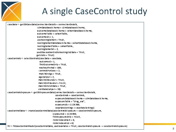
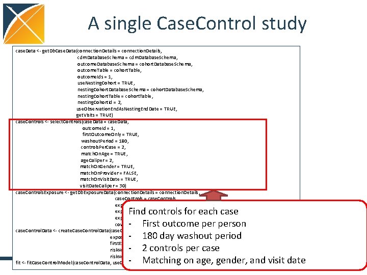
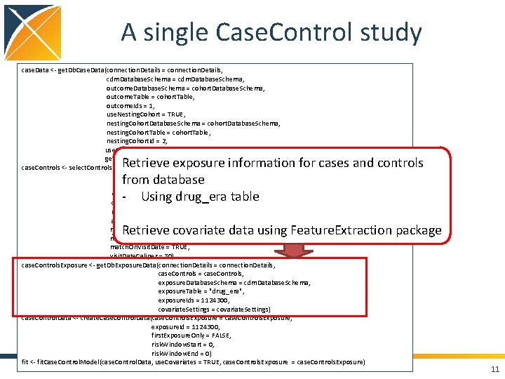
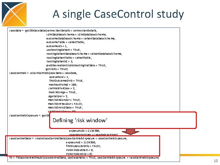
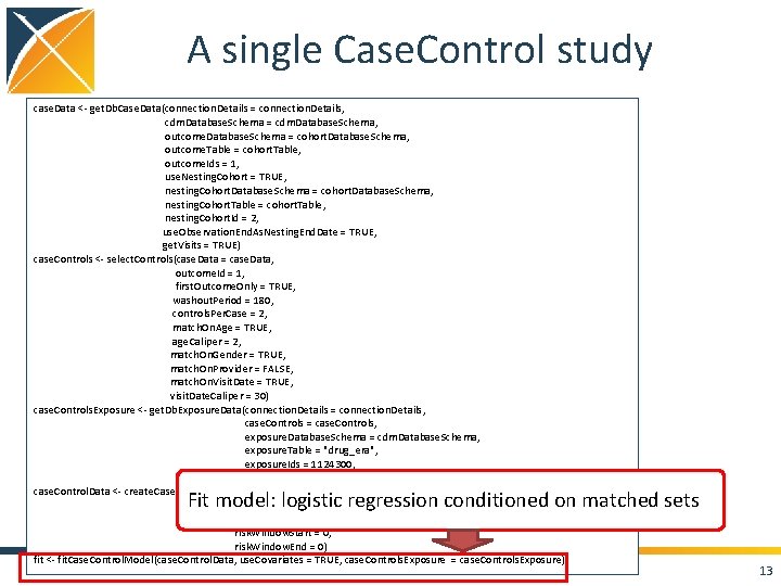
A single Case. Control study case. Data <- get. Db. Case. Data(connection. Details = connection. Details, cdm. Database. Schema = cdm. Database. Schema, outcome. Database. Schema = cohort. Database. Schema, outcome. Table = cohort. Table, outcome. Ids = 1, use. Nesting. Cohort = TRUE, nesting. Cohort. Database. Schema = cohort. Database. Schema, nesting. Cohort. Table = cohort. Table, nesting. Cohort. Id = 2, use. Observation. End. As. Nesting. End. Date = TRUE, get. Visits = TRUE) case. Controls <- select. Controls(case. Data = case. Data, outcome. Id = 1, first. Outcome. Only = TRUE, washout. Period = 180, controls. Per. Case = 2, match. On. Age = TRUE, age. Caliper = 2, match. On. Gender = TRUE, match. On. Provider = FALSE, match. On. Visit. Date = TRUE, visit. Date. Caliper = 30) case. Controls. Exposure <- get. Db. Exposure. Data(connection. Details = connection. Details, case. Controls = case. Controls, exposure. Database. Schema = cdm. Database. Schema, exposure. Table = "drug_era", exposure. Ids = 1124300, covariate. Settings = covariate. Settings) case. Control. Data <- create. Case. Control. Data(case. Controls. Exposure = case. Controls. Exposure, exposure. Id = 1124300, first. Exposure. Only = FALSE, risk. Window. Start = 0, risk. Window. End = 0) fit <- fit. Case. Control. Model(case. Control. Data, use. Covariates = TRUE, case. Controls. Exposure = case. Controls. Exposure) 8

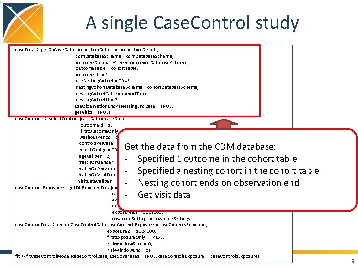
A single Case. Control study case. Data <- get. Db. Case. Data(connection. Details = connection. Details, cdm. Database. Schema = cdm. Database. Schema, outcome. Database. Schema = cohort. Database. Schema, outcome. Table = cohort. Table, outcome. Ids = 1, use. Nesting. Cohort = TRUE, nesting. Cohort. Database. Schema = cohort. Database. Schema, nesting. Cohort. Table = cohort. Table, nesting. Cohort. Id = 2, use. Observation. End. As. Nesting. End. Date = TRUE, get. Visits = TRUE) case. Controls <- select. Controls(case. Data = case. Data, outcome. Id = 1, first. Outcome. Only = TRUE, washout. Period = 180, controls. Per. Case = 2, match. On. Age = TRUE, age. Caliper = 2, match. On. Gender = TRUE, match. On. Provider = FALSE, match. On. Visit. Date = TRUE, visit. Date. Caliper = 30) case. Controls. Exposure <- get. Db. Exposure. Data(connection. Details = connection. Details, case. Controls = case. Controls, exposure. Database. Schema = cdm. Database. Schema, exposure. Table = "drug_era", exposure. Ids = 1124300, covariate. Settings = covariate. Settings) case. Control. Data <- create. Case. Control. Data(case. Controls. Exposure = case. Controls. Exposure, exposure. Id = 1124300, first. Exposure. Only = FALSE, risk. Window. Start = 0, risk. Window. End = 0) fit <- fit. Case. Control. Model(case. Control. Data, use. Covariates = TRUE, case. Controls. Exposure = case. Controls. Exposure) Get the data from the CDM database: - Specified 1 outcome in the cohort table - Specified a nesting cohort in the cohort table - Nesting cohort ends on observation end - Get visit data 9

A single Case. Control study case. Data <- get. Db. Case. Data(connection. Details = connection. Details, cdm. Database. Schema = cdm. Database. Schema, outcome. Database. Schema = cohort. Database. Schema, outcome. Table = cohort. Table, outcome. Ids = 1, use. Nesting. Cohort = TRUE, nesting. Cohort. Database. Schema = cohort. Database. Schema, nesting. Cohort. Table = cohort. Table, nesting. Cohort. Id = 2, use. Observation. End. As. Nesting. End. Date = TRUE, get. Visits = TRUE) case. Controls <- select. Controls(case. Data = case. Data, outcome. Id = 1, first. Outcome. Only = TRUE, washout. Period = 180, controls. Per. Case = 2, match. On. Age = TRUE, age. Caliper = 2, match. On. Gender = TRUE, match. On. Provider = FALSE, match. On. Visit. Date = TRUE, visit. Date. Caliper = 30) case. Controls. Exposure <- get. Db. Exposure. Data(connection. Details = connection. Details, case. Controls = case. Controls, exposure. Database. Schema = cdm. Database. Schema, exposure. Table = "drug_era", exposure. Ids = 1124300, covariate. Settings = covariate. Settings) case. Control. Data <- create. Case. Control. Data(case. Controls. Exposure = case. Controls. Exposure, exposure. Id = 1124300, first. Exposure. Only = FALSE, risk. Window. Start = 0, risk. Window. End = 0) fit <- fit. Case. Control. Model(case. Control. Data, use. Covariates = TRUE, case. Controls. Exposure = case. Controls. Exposure) Find controls for each case - First outcome person - 180 day washout period - 2 controls per case - Matching on age, gender, and visit date 10

A single Case. Control study case. Data <- get. Db. Case. Data(connection. Details = connection. Details, cdm. Database. Schema = cdm. Database. Schema, outcome. Database. Schema = cohort. Database. Schema, outcome. Table = cohort. Table, outcome. Ids = 1, use. Nesting. Cohort = TRUE, nesting. Cohort. Database. Schema = cohort. Database. Schema, nesting. Cohort. Table = cohort. Table, nesting. Cohort. Id = 2, use. Observation. End. As. Nesting. End. Date = TRUE, get. Visits = TRUE) case. Controls <- select. Controls(case. Data = case. Data, outcome. Id = 1, first. Outcome. Only = TRUE, washout. Period = 180, controls. Per. Case = 2, match. On. Age = TRUE, age. Caliper = 2, match. On. Gender = TRUE, match. On. Provider = FALSE, match. On. Visit. Date = TRUE, visit. Date. Caliper = 30) case. Controls. Exposure <- get. Db. Exposure. Data(connection. Details = connection. Details, case. Controls = case. Controls, exposure. Database. Schema = cdm. Database. Schema, exposure. Table = "drug_era", exposure. Ids = 1124300, covariate. Settings = covariate. Settings) case. Control. Data <- create. Case. Control. Data(case. Controls. Exposure = case. Controls. Exposure, exposure. Id = 1124300, first. Exposure. Only = FALSE, risk. Window. Start = 0, risk. Window. End = 0) fit <- fit. Case. Control. Model(case. Control. Data, use. Covariates = TRUE, case. Controls. Exposure = case. Controls. Exposure) Retrieve exposure information for cases and controls from database - Using drug_era table Retrieve covariate data using Feature. Extraction package 11

A single Case. Control study case. Data <- get. Db. Case. Data(connection. Details = connection. Details, cdm. Database. Schema = cdm. Database. Schema, outcome. Database. Schema = cohort. Database. Schema, outcome. Table = cohort. Table, outcome. Ids = 1, use. Nesting. Cohort = TRUE, nesting. Cohort. Database. Schema = cohort. Database. Schema, nesting. Cohort. Table = cohort. Table, nesting. Cohort. Id = 2, use. Observation. End. As. Nesting. End. Date = TRUE, get. Visits = TRUE) case. Controls <- select. Controls(case. Data = case. Data, outcome. Id = 1, first. Outcome. Only = TRUE, washout. Period = 180, controls. Per. Case = 2, match. On. Age = TRUE, age. Caliper = 2, match. On. Gender = TRUE, match. On. Provider = FALSE, match. On. Visit. Date = TRUE, visit. Date. Caliper = 30) case. Controls. Exposure <- get. Db. Exposure. Data(connection. Details = connection. Details, case. Controls = case. Controls, exposure. Database. Schema = cdm. Database. Schema, exposure. Table = "drug_era", exposure. Ids = 1124300, covariate. Settings = covariate. Settings) case. Control. Data <- create. Case. Control. Data(case. Controls. Exposure = case. Controls. Exposure, exposure. Id = 1124300, first. Exposure. Only = FALSE, risk. Window. Start = 0, risk. Window. End = 0) fit <- fit. Case. Control. Model(case. Control. Data, use. Covariates = TRUE, case. Controls. Exposure = case. Controls. Exposure) Defining ‘risk window’ 12

A single Case. Control study case. Data <- get. Db. Case. Data(connection. Details = connection. Details, cdm. Database. Schema = cdm. Database. Schema, outcome. Database. Schema = cohort. Database. Schema, outcome. Table = cohort. Table, outcome. Ids = 1, use. Nesting. Cohort = TRUE, nesting. Cohort. Database. Schema = cohort. Database. Schema, nesting. Cohort. Table = cohort. Table, nesting. Cohort. Id = 2, use. Observation. End. As. Nesting. End. Date = TRUE, get. Visits = TRUE) case. Controls <- select. Controls(case. Data = case. Data, outcome. Id = 1, first. Outcome. Only = TRUE, washout. Period = 180, controls. Per. Case = 2, match. On. Age = TRUE, age. Caliper = 2, match. On. Gender = TRUE, match. On. Provider = FALSE, match. On. Visit. Date = TRUE, visit. Date. Caliper = 30) case. Controls. Exposure <- get. Db. Exposure. Data(connection. Details = connection. Details, case. Controls = case. Controls, exposure. Database. Schema = cdm. Database. Schema, exposure. Table = "drug_era", exposure. Ids = 1124300, covariate. Settings = covariate. Settings) case. Control. Data <- create. Case. Control. Data(case. Controls. Exposure = case. Controls. Exposure, exposure. Id = 1124300, first. Exposure. Only = FALSE, risk. Window. Start = 0, risk. Window. End = 0) fit <- fit. Case. Control. Model(case. Control. Data, use. Covariates = TRUE, case. Controls. Exposure = case. Controls. Exposure) Fit model: logistic regression conditioned on matched sets 13

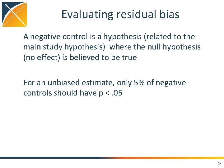
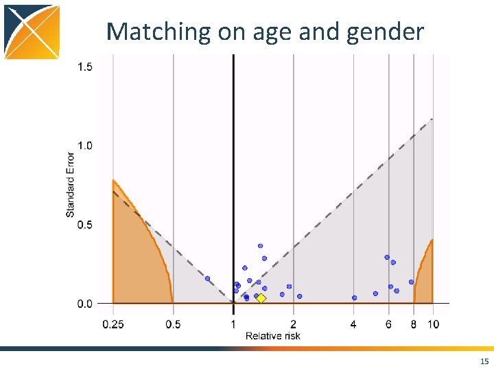
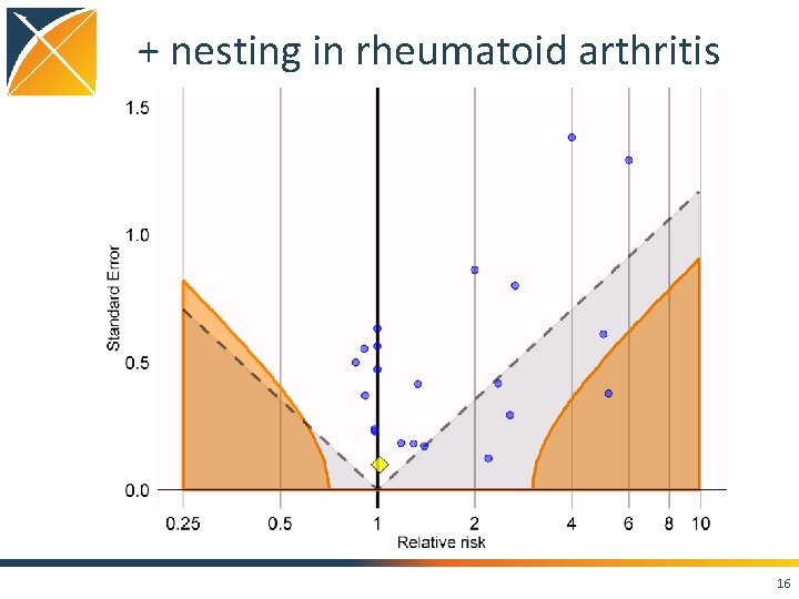
Evaluating residual bias A negative control is a hypothesis (related to the main study hypothesis) where the null hypothesis (no effect) is believed to be true For an unbiased estimate, only 5% of negative controls should have p <. 05 14

Matching on age and gender 15

+ nesting in rheumatoid arthritis 16

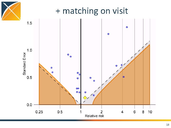
+ adding Charlson, DCSI, and CHADS 2 17

+ matching on visit 18

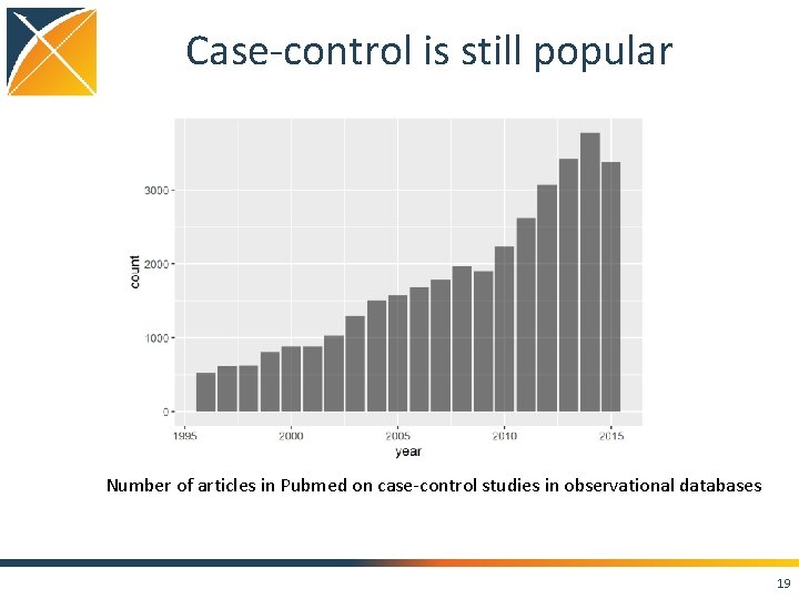
Case-control is still popular Number of articles in Pubmed on case-control studies in observational databases 19

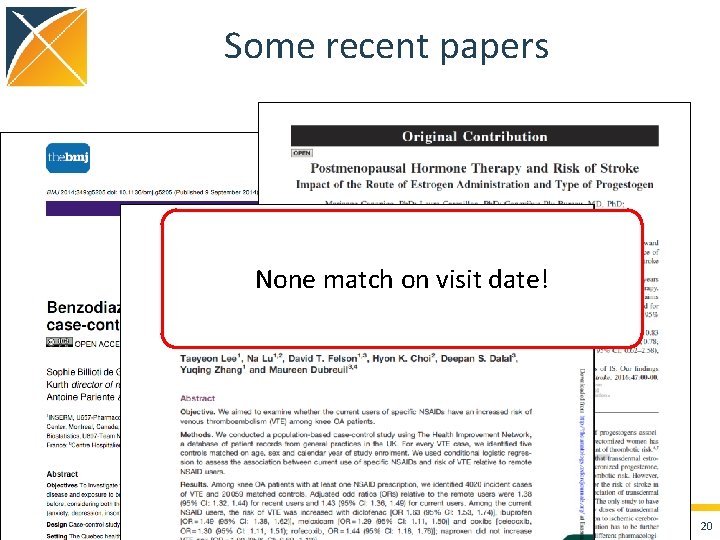
Some recent papers None match on visit date! 20

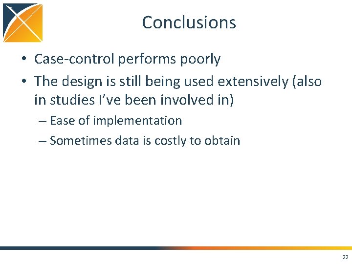
Conclusions • Case. Control package features – Matching on • • • Calendar time Age Gender Visit dates Provider – Nesting – Covariates • Using negative controls, we still see residual bias even when nesting, matching, and adding covariates • Strongly positively biased when not matching on visit 21

Conclusions • Case-control performs poorly • The design is still being used extensively (also in studies I’ve been involved in) – Ease of implementation – Sometimes data is costly to obtain 22

Next steps • Writing a paper arguing against case-control in retrospective observational data 23

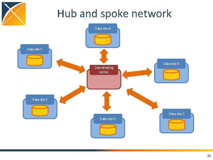
Distributed research network • Many observational databases in OHDSI – large numbers – large diversity • We cannot share patient-level data • Solution: – analysis code ‘visits’ the data – only population-level data is shared 24

Hub and spoke network Data site A Data site F Coordinating center Data site B Data site E Data site C Data site D 25

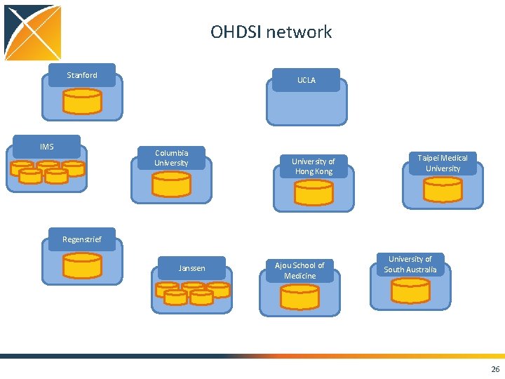
OHDSI network Stanford IMS UCLA Columbia University of Hong Kong Taipei Medical University Regenstrief Janssen Ajou School of Medicine University of South Australia 26

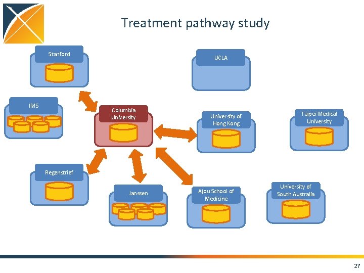
Treatment pathway study Stanford IMS UCLA Columbia University of Hong Kong Taipei Medical University Regenstrief Janssen Ajou School of Medicine University of South Australia 27

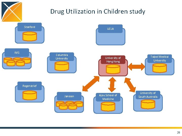
Drug Utilization in Children study Stanford IMS UCLA Columbia University of Hong Kong Taipei Medical University Regenstrief Janssen Ajou School of Medicine University of South Australia 28

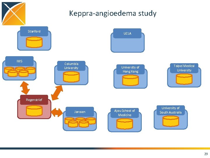
Keppra-angioedema study Stanford IMS UCLA Columbia University of Hong Kong Taipei Medical University Regenstrief Janssen Ajou School of Medicine University of South Australia 29

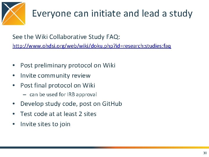
Everyone can initiate and lead a study See the Wiki Collaborative Study FAQ: http: //www. ohdsi. org/web/wiki/doku. php? id=research: studies: faq • Post preliminary protocol on Wiki • Invite community review • Post final protocol on Wiki – can be used for IRB approval • Develop study code, post on Git. Hub • Test code at at least 2 sites • Invite sites to join 30

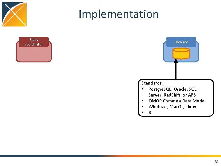
Implementation Study coordinator Data site Standards: • Postgre. SQL, Oracle, SQL Server, Red. Shift, or APS • OMOP Common Data Model • Windows, Mac. Os, Linux • R 31

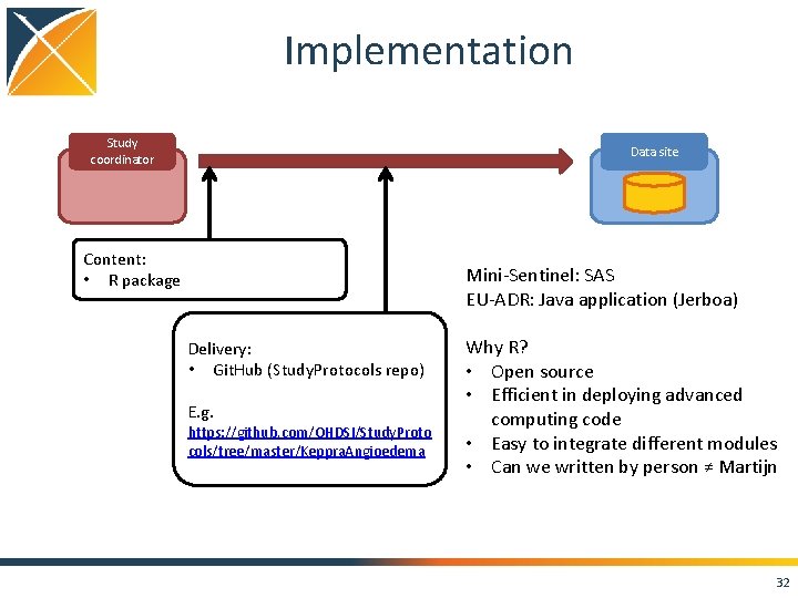
Implementation Study coordinator Data site Content: • R package Mini-Sentinel: SAS EU-ADR: Java application (Jerboa) Delivery: • Git. Hub (Study. Protocols repo) E. g. https: //github. com/OHDSI/Study. Proto cols/tree/master/Keppra. Angioedema Why R? • Open source • Efficient in deploying advanced computing code • Easy to integrate different modules • Can we written by person ≠ Martijn 32

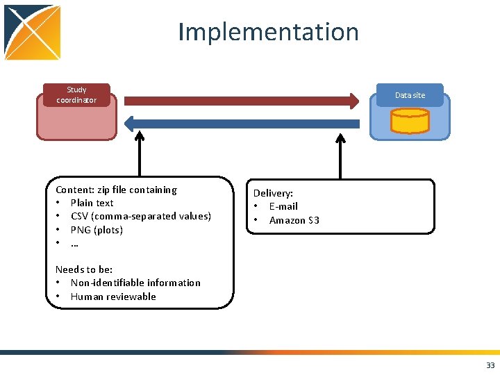
Implementation Study coordinator Content: zip file containing • Plain text • CSV (comma-separated values) • PNG (plots) • … Data site Delivery: • E-mail • Amazon S 3 Needs to be: • Non-identifiable information • Human reviewable 33

Interpreting results of a network study Options: • Do not combine results from sites • Combine results from sites using meta-analytic approach • Run a single regression across sites 34

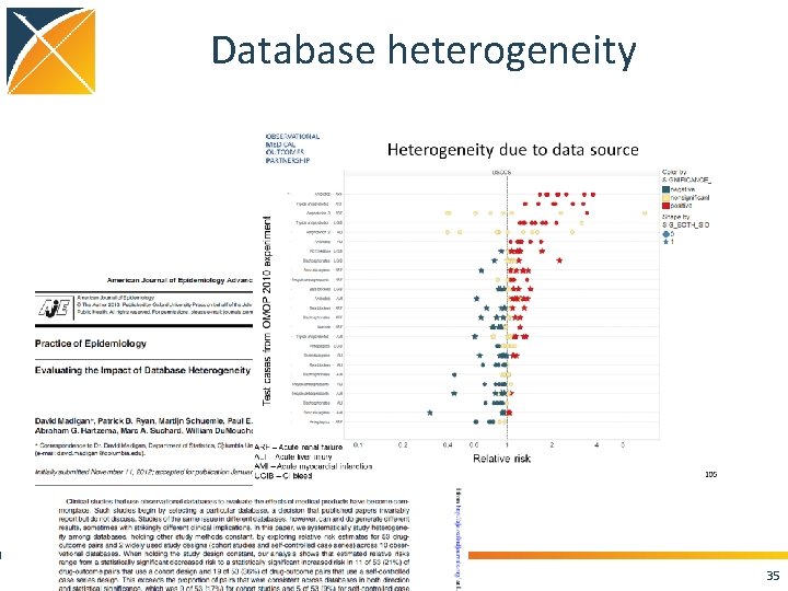
Database heterogeneity 35

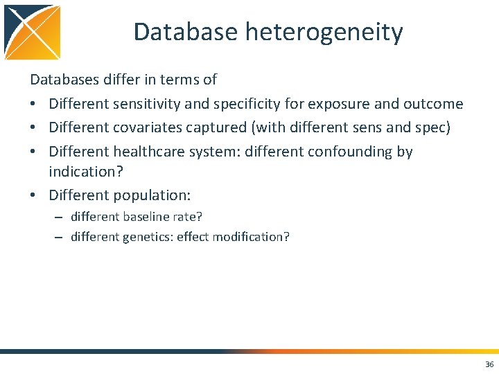
Database heterogeneity Databases differ in terms of • Different sensitivity and specificity for exposure and outcome • Different covariates captured (with different sens and spec) • Different healthcare system: different confounding by indication? • Different population: – different baseline rate? – different genetics: effect modification? 36

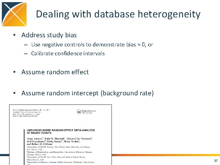
Dealing with database heterogeneity • Address study bias – Use negative controls to demonstrate bias ≈ 0, or – Calibrate confidence intervals • Assume random effect • Assume random intercept (background rate) 37

Conclusions • Starting to think about network studies 38

Topic of next meeting(s)? • ? 39

Next workgroup meeting July 13 • 3 pm Hong Kong / Taiwan • 4 pm South Korea • 4: 30 pm Adelaide • 9 am Central European time http: //www. ohdsi. org/web/wiki/doku. php? id=projects: workgroups: est-methods 40