Self Controlled Case Series package Martijn Schuemie Marc




- Slides: 27

Self. Controlled. Case. Series package Martijn Schuemie, Marc Suchard, Patrick Ryan

Quick recap of previous meeting • We discussed the Cohort. Method package – Large scale regression propensity models – Large scale regression outcome models – Using negative controls, we see a reduction in residual bias when using PS matching + full outcome model • Interest to learn about the other methods packages as well

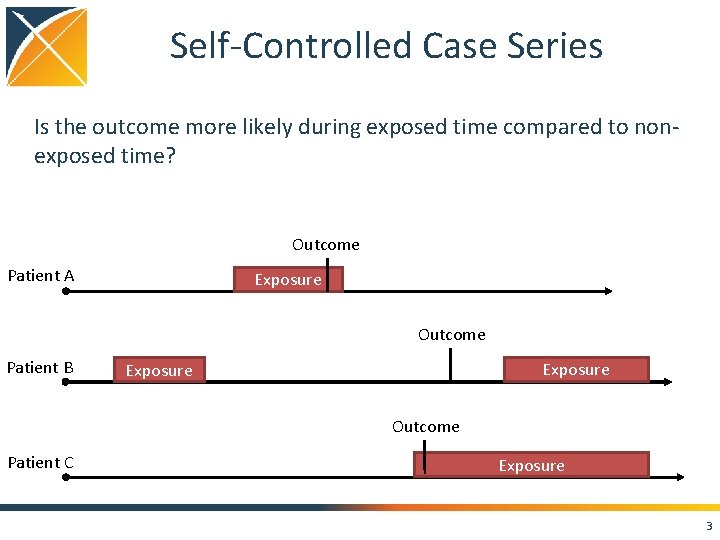
Self-Controlled Case Series Is the outcome more likely during exposed time compared to nonexposed time? Outcome Patient A Exposure Outcome Patient B Exposure Outcome Patient C Exposure 3

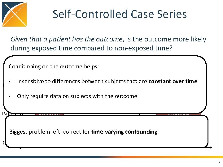
Self-Controlled Case Series Given that a patient has the outcome, is the outcome more likely during exposed time compared to non-exposed time? Conditioning on the outcome helps: Outcome - Insensitive to differences between subjects that are constant over time - Only require data on subjects with the outcome Patient A Exposure Outcome Patient B Exposure Biggest problem left: correct for time-varying. Outcome confounding Patient C Exposure 4

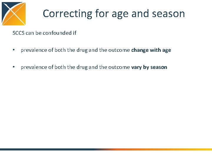
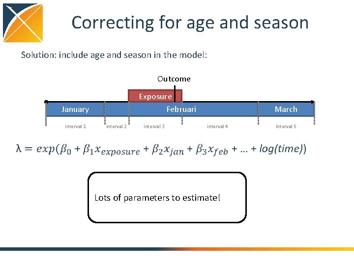
Correcting for age and season SCCS can be confounded if • prevalence of both the drug and the outcome change with age • prevalence of both the drug and the outcome vary by season

Correcting for age and season Solution: include age and season in the model: Outcome Exposure Februari January interval 1 interval 2 interval 3 March interval 4 Lots of parameters to estimate! interval 5

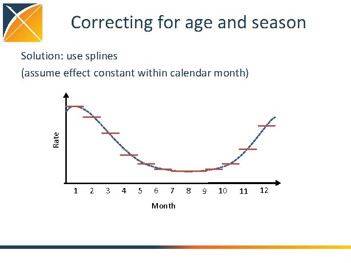
Correcting for age and season Rate Solution: use splines (assume effect constant within calendar month) 1 2 3 4 5 6 7 Month 8 9 10 11 12

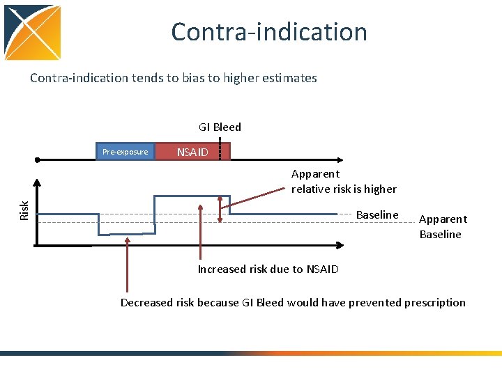
Contra-indication tends to bias to higher estimates GI Bleed Pre-exposure NSAID Risk Apparent relative risk is higher Baseline Apparent Baseline Increased risk due to NSAID Decreased risk because GI Bleed would have prevented prescription

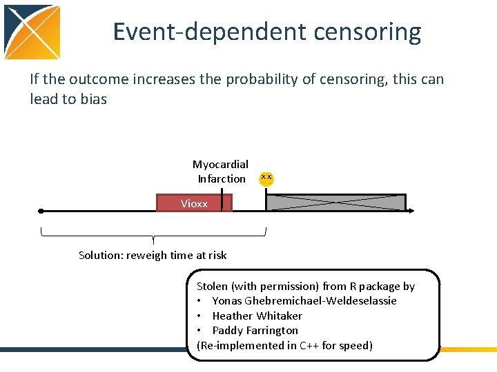
Event-dependent censoring If the outcome increases the probability of censoring, this can lead to bias Myocardial Infarction Vioxx Solution: reweigh time at risk Stolen (with permission) from R package by • Yonas Ghebremichael-Weldeselassie • Heather Whitaker • Paddy Farrington (Re-implemented in C++ for speed)

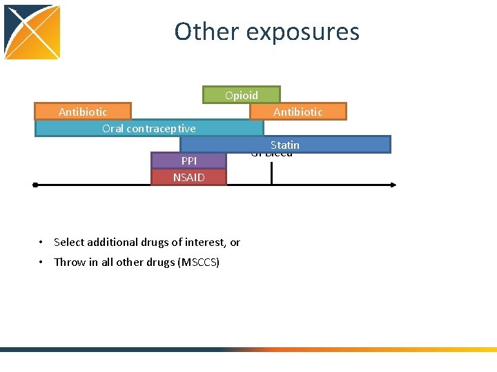
Other exposures Opioid Antibiotic Oral contraceptive PPI NSAID • Select additional drugs of interest, or • Throw in all other drugs (MSCCS) Antibiotic Statin GI Bleed

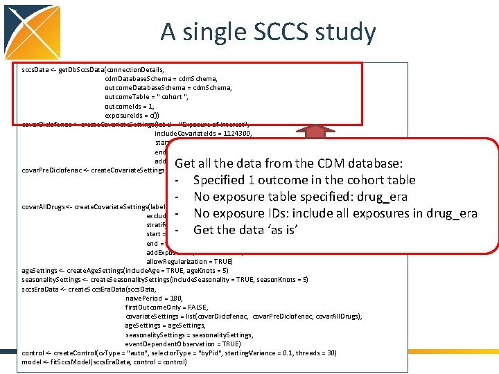
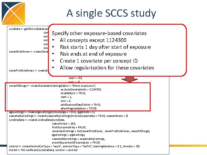
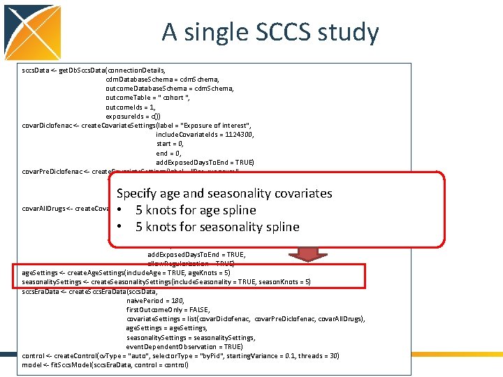
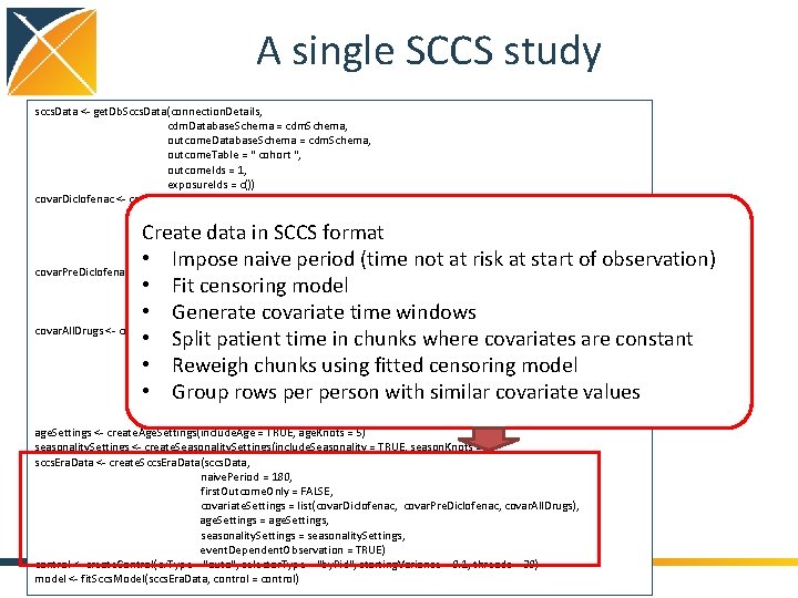
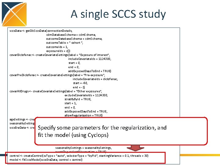
A single SCCS study sccs. Data <- get. Db. Sccs. Data(connection. Details, cdm. Database. Schema = cdm. Schema, outcome. Table = " cohort ", outcome. Ids = 1, exposure. Ids = c()) covar. Diclofenac <- create. Covariate. Settings(label = "Exposure of interest", include. Covariate. Ids = 1124300, start = 0, end = 0, add. Exposed. Days. To. End = TRUE) covar. Pre. Diclofenac <- create. Covariate. Settings(label = "Pre-exposure", include. Covariate. Ids = diclofenac, start = -60, end = -1) covar. All. Drugs <- create. Covariate. Settings(label = "Other exposures", exclude. Covariate. Ids = 1124300, stratify. By. Id = TRUE, start = 1, end = 0, add. Exposed. Days. To. End = TRUE, allow. Regularization = TRUE) age. Settings <- create. Age. Settings(include. Age = TRUE, age. Knots = 5) seasonality. Settings <- create. Seasonality. Settings(include. Seasonality = TRUE, season. Knots = 5) sccs. Era. Data <- create. Sccs. Era. Data(sccs. Data, naive. Period = 180, first. Outcome. Only = FALSE, covariate. Settings = list(covar. Diclofenac, covar. Pre. Diclofenac, covar. All. Drugs), age. Settings = age. Settings, seasonality. Settings = seasonality. Settings, event. Dependent. Observation = TRUE) control <- create. Control(cv. Type = "auto", selector. Type = "by. Pid", starting. Variance = 0. 1, threads = 30) model <- fit. Sccs. Model(sccs. Era. Data, control = control)

A single SCCS study sccs. Data <- get. Db. Sccs. Data(connection. Details, cdm. Database. Schema = cdm. Schema, outcome. Table = " cohort ", outcome. Ids = 1, exposure. Ids = c()) covar. Diclofenac <- create. Covariate. Settings(label = "Exposure of interest", include. Covariate. Ids = 1124300, start = 0, end = 0, add. Exposed. Days. To. End = TRUE) covar. Pre. Diclofenac <- create. Covariate. Settings(label = "Pre-exposure", include. Covariate. Ids = diclofenac, start = -60, end = -1) covar. All. Drugs <- create. Covariate. Settings(label = "Other exposures", exclude. Covariate. Ids = 1124300, stratify. By. Id = TRUE, start = 1, end = 0, add. Exposed. Days. To. End = TRUE, allow. Regularization = TRUE) age. Settings <- create. Age. Settings(include. Age = TRUE, age. Knots = 5) seasonality. Settings <- create. Seasonality. Settings(include. Seasonality = TRUE, season. Knots = 5) sccs. Era. Data <- create. Sccs. Era. Data(sccs. Data, naive. Period = 180, first. Outcome. Only = FALSE, covariate. Settings = list(covar. Diclofenac, covar. Pre. Diclofenac, covar. All. Drugs), age. Settings = age. Settings, seasonality. Settings = seasonality. Settings, event. Dependent. Observation = TRUE) control <- create. Control(cv. Type = "auto", selector. Type = "by. Pid", starting. Variance = 0. 1, threads = 30) model <- fit. Sccs. Model(sccs. Era. Data, control = control) Get all the data from the CDM database: - Specified 1 outcome in the cohort table - No exposure table specified: drug_era - No exposure IDs: include all exposures in drug_era - Get the data ‘as is’

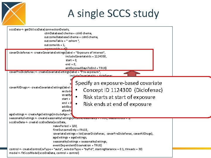
A single SCCS study sccs. Data <- get. Db. Sccs. Data(connection. Details, cdm. Database. Schema = cdm. Schema, outcome. Table = " cohort ", outcome. Ids = 1, exposure. Ids = c()) covar. Diclofenac <- create. Covariate. Settings(label = "Exposure of interest", include. Covariate. Ids = 1124300, start = 0, end = 0, add. Exposed. Days. To. End = TRUE) covar. Pre. Diclofenac <- create. Covariate. Settings(label = "Pre-exposure", include. Covariate. Ids = diclofenac, start = -60, end = -1) covar. All. Drugs <- create. Covariate. Settings(label = "Other exposures", exclude. Covariate. Ids = 1124300, stratify. By. Id = TRUE, start = 1, end = 0, add. Exposed. Days. To. End = TRUE, allow. Regularization = TRUE) age. Settings <- create. Age. Settings(include. Age = TRUE, age. Knots = 5) seasonality. Settings <- create. Seasonality. Settings(include. Seasonality = TRUE, season. Knots = 5) sccs. Era. Data <- create. Sccs. Era. Data(sccs. Data, naive. Period = 180, first. Outcome. Only = FALSE, covariate. Settings = list(covar. Diclofenac, covar. Pre. Diclofenac, covar. All. Drugs), age. Settings = age. Settings, seasonality. Settings = seasonality. Settings, event. Dependent. Observation = TRUE) control <- create. Control(cv. Type = "auto", selector. Type = "by. Pid", starting. Variance = 0. 1, threads = 30) model <- fit. Sccs. Model(sccs. Era. Data, control = control) Specify an exposure-based covariate • Concept ID 1124300 (Diclofenac) • Risk starts at start of exposure • Risk ends at end of exposure

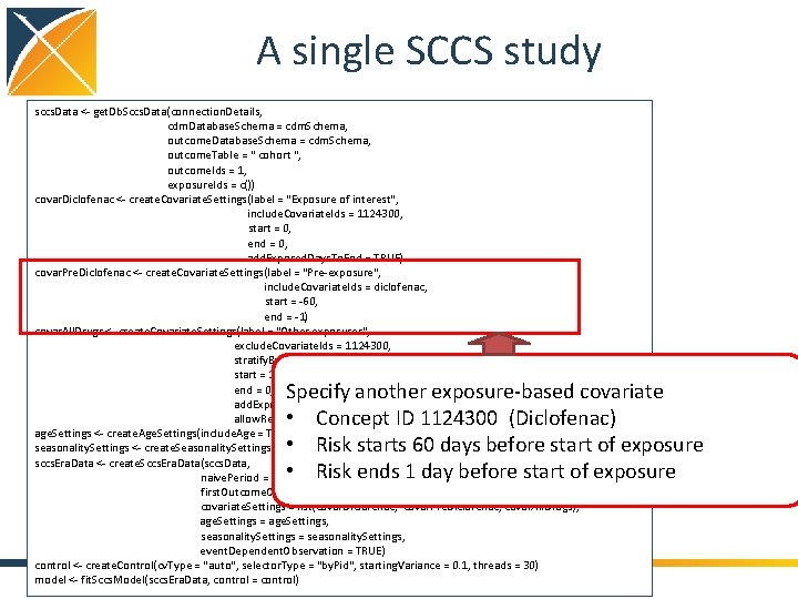
A single SCCS study sccs. Data <- get. Db. Sccs. Data(connection. Details, cdm. Database. Schema = cdm. Schema, outcome. Table = " cohort ", outcome. Ids = 1, exposure. Ids = c()) covar. Diclofenac <- create. Covariate. Settings(label = "Exposure of interest", include. Covariate. Ids = 1124300, start = 0, end = 0, add. Exposed. Days. To. End = TRUE) covar. Pre. Diclofenac <- create. Covariate. Settings(label = "Pre-exposure", include. Covariate. Ids = diclofenac, start = -60, end = -1) covar. All. Drugs <- create. Covariate. Settings(label = "Other exposures", exclude. Covariate. Ids = 1124300, stratify. By. Id = TRUE, start = 1, end = 0, add. Exposed. Days. To. End = TRUE, allow. Regularization = TRUE) age. Settings <- create. Age. Settings(include. Age = TRUE, age. Knots = 5) seasonality. Settings <- create. Seasonality. Settings(include. Seasonality = TRUE, season. Knots = 5) sccs. Era. Data <- create. Sccs. Era. Data(sccs. Data, naive. Period = 180, first. Outcome. Only = FALSE, covariate. Settings = list(covar. Diclofenac, covar. Pre. Diclofenac, covar. All. Drugs), age. Settings = age. Settings, seasonality. Settings = seasonality. Settings, event. Dependent. Observation = TRUE) control <- create. Control(cv. Type = "auto", selector. Type = "by. Pid", starting. Variance = 0. 1, threads = 30) model <- fit. Sccs. Model(sccs. Era. Data, control = control) Specify another exposure-based covariate • Concept ID 1124300 (Diclofenac) • Risk starts 60 days before start of exposure • Risk ends 1 day before start of exposure

A single SCCS study sccs. Data <- get. Db. Sccs. Data(connection. Details, cdm. Database. Schema = cdm. Schema, outcome. Table = " cohort ", outcome. Ids = 1, exposure. Ids = c()) covar. Diclofenac <- create. Covariate. Settings(label = "Exposure of interest", include. Covariate. Ids = 1124300, start = 0, end = 0, add. Exposed. Days. To. End = TRUE) covar. Pre. Diclofenac <- create. Covariate. Settings(label = "Pre-exposure", include. Covariate. Ids = diclofenac, start = -60, end = -1) covar. All. Drugs <- create. Covariate. Settings(label = "Other exposures", exclude. Covariate. Ids = 1124300, stratify. By. Id = TRUE, start = 1, end = 0, add. Exposed. Days. To. End = TRUE, allow. Regularization = TRUE) age. Settings <- create. Age. Settings(include. Age = TRUE, age. Knots = 5) seasonality. Settings <- create. Seasonality. Settings(include. Seasonality = TRUE, season. Knots = 5) sccs. Era. Data <- create. Sccs. Era. Data(sccs. Data, naive. Period = 180, first. Outcome. Only = FALSE, covariate. Settings = list(covar. Diclofenac, covar. Pre. Diclofenac, covar. All. Drugs), age. Settings = age. Settings, seasonality. Settings = seasonality. Settings, event. Dependent. Observation = TRUE) control <- create. Control(cv. Type = "auto", selector. Type = "by. Pid", starting. Variance = 0. 1, threads = 30) model <- fit. Sccs. Model(sccs. Era. Data, control = control) Specify other exposure-based covariates • All concepts except 1124300 • Risk starts 1 day after start of exposure • Risk ends at end of exposure • Create 1 covariate per concept ID • Allow regularization for these covariates

A single SCCS study sccs. Data <- get. Db. Sccs. Data(connection. Details, cdm. Database. Schema = cdm. Schema, outcome. Table = " cohort ", outcome. Ids = 1, exposure. Ids = c()) covar. Diclofenac <- create. Covariate. Settings(label = "Exposure of interest", include. Covariate. Ids = 1124300, start = 0, end = 0, add. Exposed. Days. To. End = TRUE) covar. Pre. Diclofenac <- create. Covariate. Settings(label = "Pre-exposure", include. Covariate. Ids = diclofenac, start = -60, end = -1) covar. All. Drugs <- create. Covariate. Settings(label = "Other exposures", exclude. Covariate. Ids = 1124300, stratify. By. Id = TRUE, start = 1, end = 0, add. Exposed. Days. To. End = TRUE, allow. Regularization = TRUE) age. Settings <- create. Age. Settings(include. Age = TRUE, age. Knots = 5) seasonality. Settings <- create. Seasonality. Settings(include. Seasonality = TRUE, season. Knots = 5) sccs. Era. Data <- create. Sccs. Era. Data(sccs. Data, naive. Period = 180, first. Outcome. Only = FALSE, covariate. Settings = list(covar. Diclofenac, covar. Pre. Diclofenac, covar. All. Drugs), age. Settings = age. Settings, seasonality. Settings = seasonality. Settings, event. Dependent. Observation = TRUE) control <- create. Control(cv. Type = "auto", selector. Type = "by. Pid", starting. Variance = 0. 1, threads = 30) model <- fit. Sccs. Model(sccs. Era. Data, control = control) Specify age and seasonality covariates • 5 knots for age spline • 5 knots for seasonality spline

A single SCCS study sccs. Data <- get. Db. Sccs. Data(connection. Details, cdm. Database. Schema = cdm. Schema, outcome. Table = " cohort ", outcome. Ids = 1, exposure. Ids = c()) covar. Diclofenac <- create. Covariate. Settings(label = "Exposure of interest", include. Covariate. Ids = 1124300, start = 0, end = 0, add. Exposed. Days. To. End = TRUE) covar. Pre. Diclofenac <- create. Covariate. Settings(label = "Pre-exposure", include. Covariate. Ids = diclofenac, start = -60, end = -1) covar. All. Drugs <- create. Covariate. Settings(label = "Other exposures", exclude. Covariate. Ids = 1124300, stratify. By. Id = TRUE, start = 1, end = 0, add. Exposed. Days. To. End = TRUE, allow. Regularization = TRUE) age. Settings <- create. Age. Settings(include. Age = TRUE, age. Knots = 5) seasonality. Settings <- create. Seasonality. Settings(include. Seasonality = TRUE, season. Knots = 5) sccs. Era. Data <- create. Sccs. Era. Data(sccs. Data, naive. Period = 180, first. Outcome. Only = FALSE, covariate. Settings = list(covar. Diclofenac, covar. Pre. Diclofenac, covar. All. Drugs), age. Settings = age. Settings, seasonality. Settings = seasonality. Settings, event. Dependent. Observation = TRUE) control <- create. Control(cv. Type = "auto", selector. Type = "by. Pid", starting. Variance = 0. 1, threads = 30) model <- fit. Sccs. Model(sccs. Era. Data, control = control) Create data in SCCS format • Impose naive period (time not at risk at start of observation) • Fit censoring model • Generate covariate time windows • Split patient time in chunks where covariates are constant • Reweigh chunks using fitted censoring model • Group rows person with similar covariate values

A single SCCS study sccs. Data <- get. Db. Sccs. Data(connection. Details, cdm. Database. Schema = cdm. Schema, outcome. Table = " cohort ", outcome. Ids = 1, exposure. Ids = c()) covar. Diclofenac <- create. Covariate. Settings(label = "Exposure of interest", include. Covariate. Ids = 1124300, start = 0, end = 0, add. Exposed. Days. To. End = TRUE) covar. Pre. Diclofenac <- create. Covariate. Settings(label = "Pre-exposure", include. Covariate. Ids = diclofenac, start = -60, end = -1) covar. All. Drugs <- create. Covariate. Settings(label = "Other exposures", exclude. Covariate. Ids = 1124300, stratify. By. Id = TRUE, start = 1, end = 0, add. Exposed. Days. To. End = TRUE, allow. Regularization = TRUE) age. Settings <- create. Age. Settings(include. Age = TRUE, age. Knots = 5) seasonality. Settings <- create. Seasonality. Settings(include. Seasonality = TRUE, season. Knots = 5) sccs. Era. Data <- create. Sccs. Era. Data(sccs. Data, naive. Period = 180, first. Outcome. Only = FALSE, covariate. Settings = list(covar. Diclofenac, covar. Pre. Diclofenac, covar. All. Drugs), age. Settings = age. Settings, seasonality. Settings = seasonality. Settings, event. Dependent. Observation = TRUE) control <- create. Control(cv. Type = "auto", selector. Type = "by. Pid", starting. Variance = 0. 1, threads = 30) model <- fit. Sccs. Model(sccs. Era. Data, control = control) Specify some parameters for the regularization, and fit the model (using Cyclops)

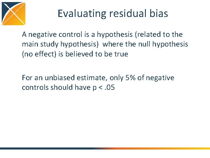
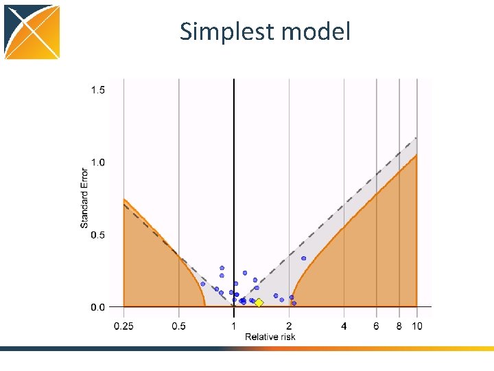
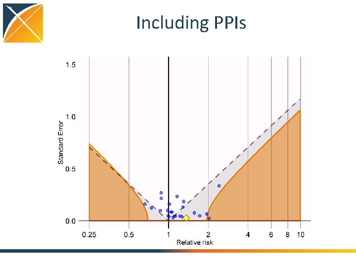
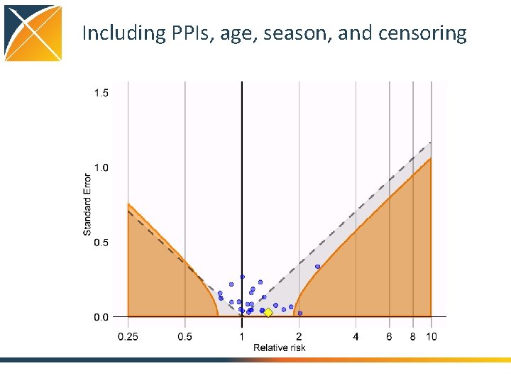
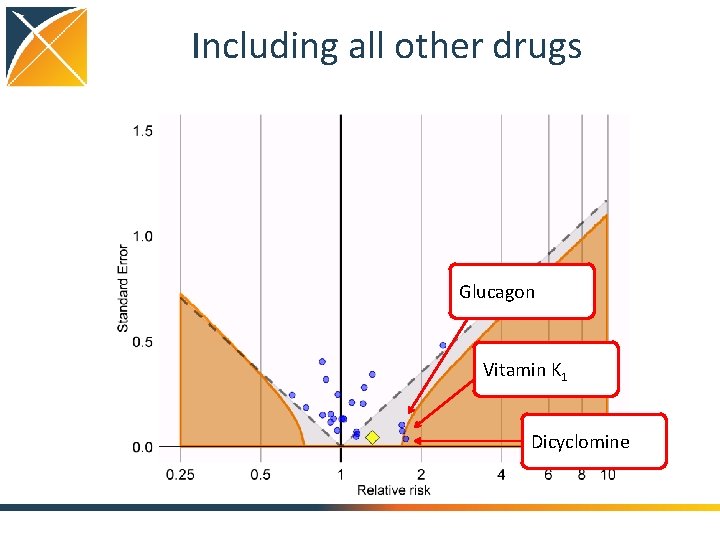
Evaluating residual bias A negative control is a hypothesis (related to the main study hypothesis) where the null hypothesis (no effect) is believed to be true For an unbiased estimate, only 5% of negative controls should have p <. 05

Simplest model

Including PPIs

Including PPIs, age, season, and censoring

Including all other drugs Glucagon Vitamin K 1 Dicyclomine

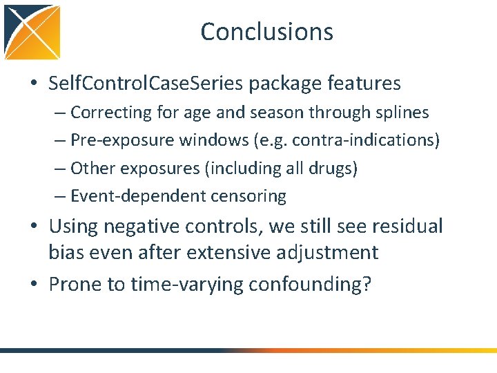
Conclusions • Self. Control. Case. Series package features – Correcting for age and season through splines – Pre-exposure windows (e. g. contra-indications) – Other exposures (including all drugs) – Event-dependent censoring • Using negative controls, we still see residual bias even after extensive adjustment • Prone to time-varying confounding?

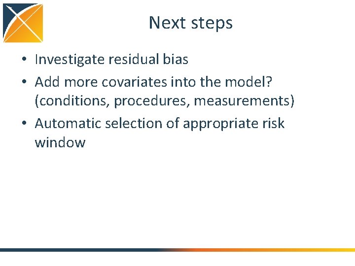
Next steps • Investigate residual bias • Add more covariates into the model? (conditions, procedures, measurements) • Automatic selection of appropriate risk window

Topic of next meeting(s)? • Method evaluation • Identifying the important questions that can be answered using observational research • TMU’s web-based case-control study app • ? 26

Next workgroup meeting June 1 st • 3 pm Hong Kong / Taiwan • 4 pm South Korea • 4: 30 pm Adelaide • 9 am Central European time http: //www. ohdsi. org/web/wiki/doku. php? id=projects: workgroups: est-methods 27