Cohort Method package Martijn Schuemie Marc Suchard Patrick




- Slides: 34

Cohort. Method package Martijn Schuemie, Marc Suchard, Patrick Ryan

Quick recap of previous meeting • Western hemisphere meeting cancelled due to lack of interest • We discussed the OHDSI Methods Library – – New-user cohort method using propensity scores Self-Controlled Case Series Self-Controlled Cohort IC Temporal Pattern Discovery • Necessity of analysis code validation (OHDSI Best Practice™) – – Unit testing Simulation Code review Double coding • Interest in additional methods – Case-control? – Methods to deal with time-varying exposure

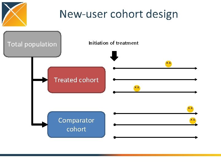
New-user cohort design Total population Initiation of treatment Treated cohort Comparator cohort

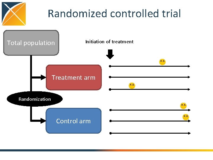
Randomized controlled trial Total population Initiation of treatment Treatment arm Randomization Control arm

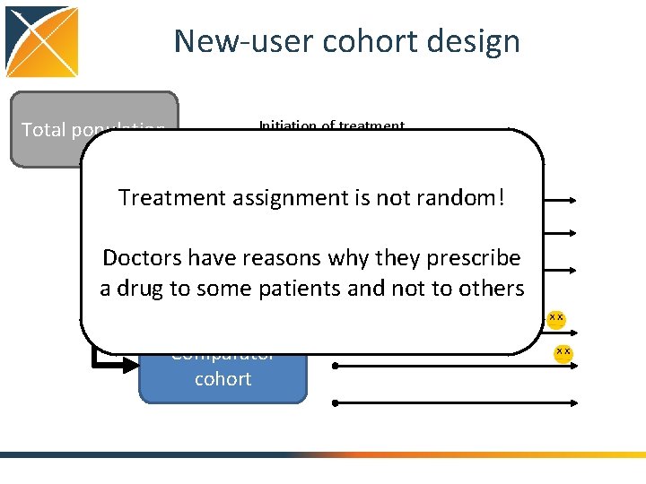
New-user cohort design Total population Initiation of treatment Treatment assignment is not random! Treated cohort Doctors have reasons why they prescribe a drug to some patients and not to others Comparator cohort

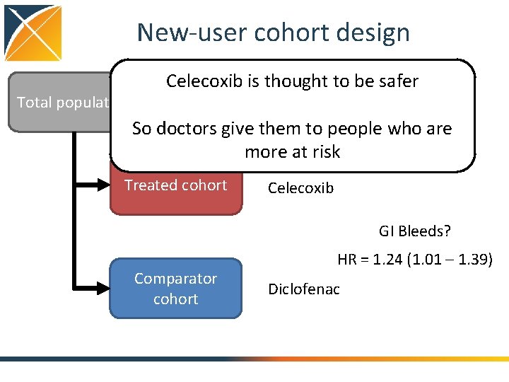
New-user cohort design Total population Celecoxib is thought to be safer So doctors give them to people who are more at risk Treated cohort Celecoxib GI Bleeds? Comparator cohort HR = 1. 24 (1. 01 – 1. 39) Diclofenac

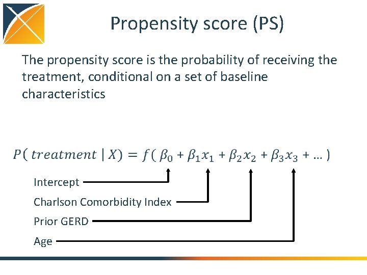
Propensity score (PS) The propensity score is the probability of receiving the treatment, conditional on a set of baseline characteristics Intercept Charlson Comorbidity Index Prior GERD Age

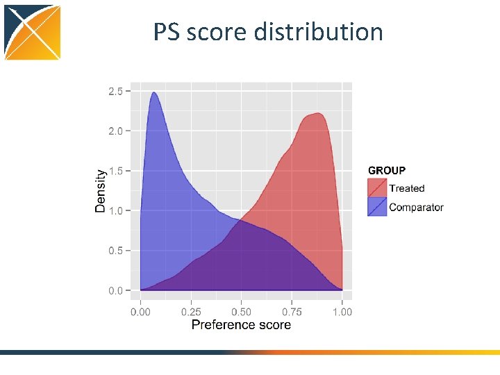
PS score distribution

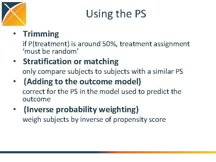
Using the PS • Trimming if P(treatment) is around 50%, treatment assignment ‘must be random’ • Stratification or matching only compare subjects to subjects with a similar PS • (Adding to the outcome model) correct for the PS in the model used to predict the outcome • (Inverse probability weighting) weigh subjects by inverse of propensity score

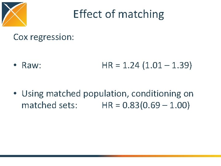
Effect of matching Cox regression: • Raw: HR = 1. 24 (1. 01 – 1. 39) • Using matched population, conditioning on matched sets: HR = 0. 83(0. 69 – 1. 00)

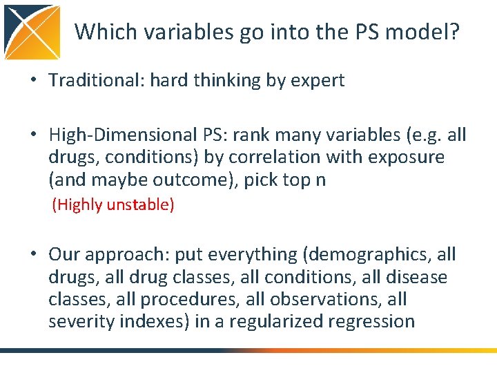
Which variables go into the PS model? • Traditional: hard thinking by expert • High-Dimensional PS: rank many variables (e. g. all drugs, conditions) by correlation with exposure (and maybe outcome), pick top n (Highly unstable) • Our approach: put everything (demographics, all drug classes, all conditions, all disease classes, all procedures, all observations, all severity indexes) in a regularized regression

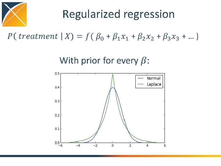
Regularized regression

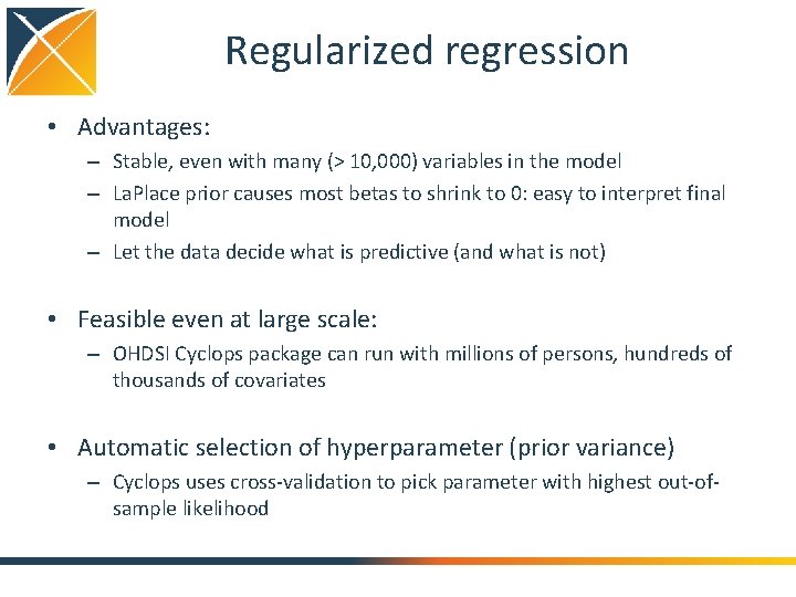
Regularized regression • Advantages: – Stable, even with many (> 10, 000) variables in the model – La. Place prior causes most betas to shrink to 0: easy to interpret final model – Let the data decide what is predictive (and what is not) • Feasible even at large scale: – OHDSI Cyclops package can run with millions of persons, hundreds of thousands of covariates • Automatic selection of hyperparameter (prior variance) – Cyclops uses cross-validation to pick parameter with highest out-ofsample likelihood

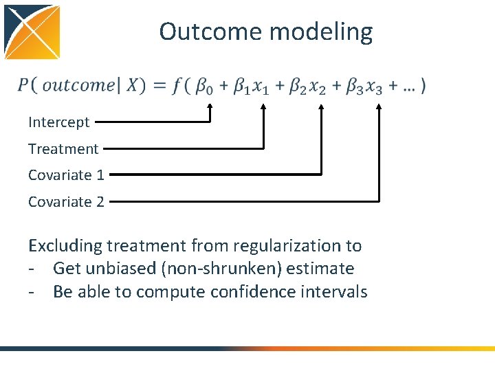
Outcome modeling Intercept Treatment Covariate 1 Covariate 2 Excluding treatment from regularization to - Get unbiased (non-shrunken) estimate - Be able to compute confidence intervals

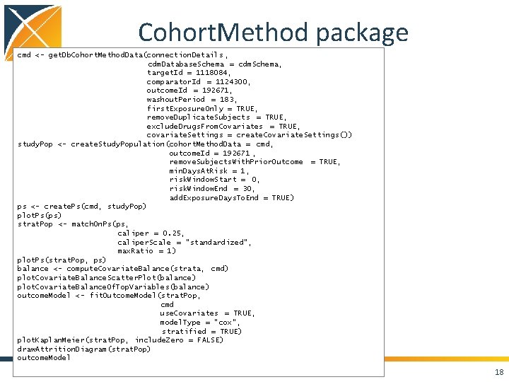
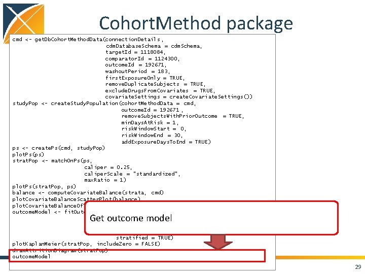
Cohort. Method package cmd <- get. Db. Cohort. Method. Data(connection. Details , cdm. Database. Schema = cdm. Schema, target. Id = 1118084, comparator. Id = 1124300, outcome. Id = 192671, washout. Period = 183, first. Exposure. Only = TRUE, remove. Duplicate. Subjects = TRUE, exclude. Drugs. From. Covariates = TRUE, covariate. Settings = create. Covariate. Settings()) study. Pop <- create. Study. Population(cohort. Method. Data = cmd, outcome. Id = 192671 , remove. Subjects. With. Prior. Outcome = TRUE, min. Days. At. Risk = 1, risk. Window. Start = 0, risk. Window. End = 30, add. Exposure. Days. To. End = TRUE) ps <- create. Ps(cmd, study. Pop) plot. Ps(ps) strat. Pop <- match. On. Ps(ps, caliper = 0. 25, caliper. Scale = "standardized", max. Ratio = 1) plot. Ps(strat. Pop, ps) balance <- compute. Covariate. Balance(strata, cmd) plot. Covariate. Balance. Scatter. Plot(balance) plot. Covariate. Balance. Of. Top. Variables(balance) outcome. Model <- fit. Outcome. Model(strat. Pop, cmd use. Covariates = TRUE, model. Type = "cox", stratified = TRUE) plot. Kaplan. Meier(strat. Pop, include. Zero = FALSE) draw. Attrition. Diagram(strat. Pop) outcome. Model 18

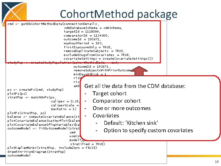
Cohort. Method package cmd <- get. Db. Cohort. Method. Data(connection. Details , cdm. Database. Schema = cdm. Schema, target. Id = 1118084, comparator. Id = 1124300, outcome. Id = 192671, washout. Period = 183, first. Exposure. Only = TRUE, remove. Duplicate. Subjects = TRUE, exclude. Drugs. From. Covariates = TRUE, covariate. Settings = create. Covariate. Settings()) study. Pop <- create. Study. Population(cohort. Method. Data = cmd, outcome. Id = 192671 , remove. Subjects. With. Prior. Outcome = TRUE, min. Days. At. Risk = 1, risk. Window. Start = 0, risk. Window. End = 30, add. Exposure. Days. To. End = TRUE) ps <- create. Ps(cmd, study. Pop) plot. Ps(ps) strat. Pop <- match. On. Ps(ps, caliper = 0. 25, caliper. Scale = "standardized", max. Ratio = 1) plot. Ps(strat. Pop, ps) balance <- compute. Covariate. Balance(strata, cmd) plot. Covariate. Balance. Scatter. Plot(balance) plot. Covariate. Balance. Of. Top. Variables(balance) outcome. Model <- fit. Outcome. Model(strat. Pop, cmd use. Covariates = TRUE, model. Type = "cox", stratified = TRUE) plot. Kaplan. Meier(strat. Pop, include. Zero = FALSE) draw. Attrition. Diagram(strat. Pop) outcome. Model Get all the data from the CDM database: - Target cohort - Comparator cohort - One or more outcomes - Covariates - Default: ‘Kitchen sink’ - Option to specify custom covariates 19

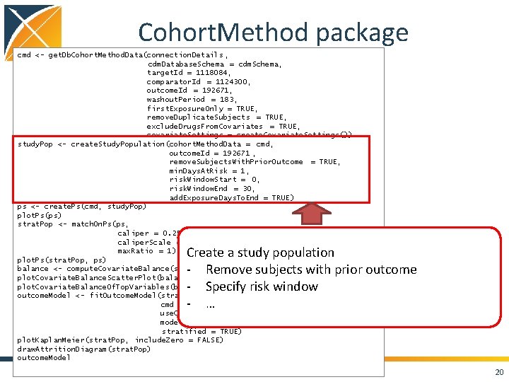
Cohort. Method package cmd <- get. Db. Cohort. Method. Data(connection. Details , cdm. Database. Schema = cdm. Schema, target. Id = 1118084, comparator. Id = 1124300, outcome. Id = 192671, washout. Period = 183, first. Exposure. Only = TRUE, remove. Duplicate. Subjects = TRUE, exclude. Drugs. From. Covariates = TRUE, covariate. Settings = create. Covariate. Settings()) study. Pop <- create. Study. Population(cohort. Method. Data = cmd, outcome. Id = 192671 , remove. Subjects. With. Prior. Outcome = TRUE, min. Days. At. Risk = 1, risk. Window. Start = 0, risk. Window. End = 30, add. Exposure. Days. To. End = TRUE) ps <- create. Ps(cmd, study. Pop) plot. Ps(ps) strat. Pop <- match. On. Ps(ps, caliper = 0. 25, caliper. Scale = "standardized", max. Ratio = 1) plot. Ps(strat. Pop, ps) balance <- compute. Covariate. Balance(strata, cmd) plot. Covariate. Balance. Scatter. Plot(balance) plot. Covariate. Balance. Of. Top. Variables(balance) outcome. Model <- fit. Outcome. Model(strat. Pop, cmd use. Covariates = TRUE, model. Type = "cox", stratified = TRUE) plot. Kaplan. Meier(strat. Pop, include. Zero = FALSE) draw. Attrition. Diagram(strat. Pop) outcome. Model Create a study population - Remove subjects with prior outcome - Specify risk window - … 20

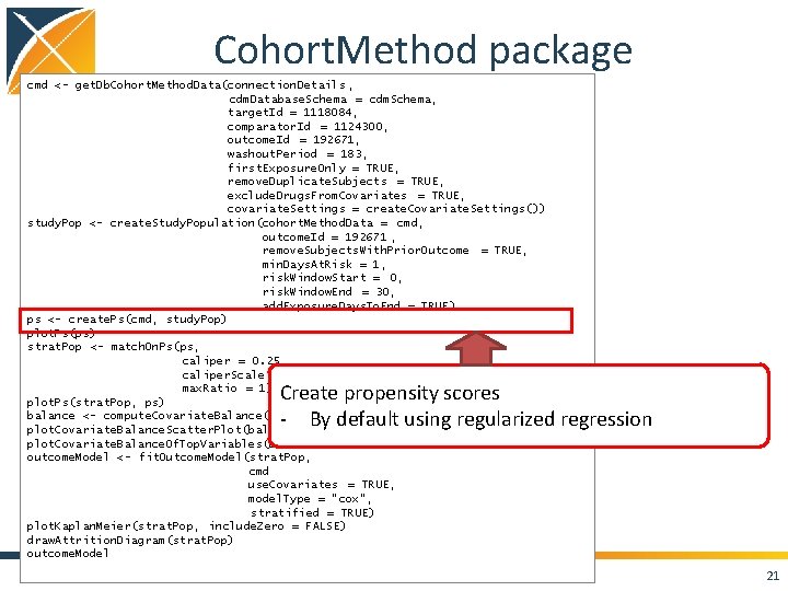
Cohort. Method package cmd <- get. Db. Cohort. Method. Data(connection. Details , cdm. Database. Schema = cdm. Schema, target. Id = 1118084, comparator. Id = 1124300, outcome. Id = 192671, washout. Period = 183, first. Exposure. Only = TRUE, remove. Duplicate. Subjects = TRUE, exclude. Drugs. From. Covariates = TRUE, covariate. Settings = create. Covariate. Settings()) study. Pop <- create. Study. Population(cohort. Method. Data = cmd, outcome. Id = 192671 , remove. Subjects. With. Prior. Outcome = TRUE, min. Days. At. Risk = 1, risk. Window. Start = 0, risk. Window. End = 30, add. Exposure. Days. To. End = TRUE) ps <- create. Ps(cmd, study. Pop) plot. Ps(ps) strat. Pop <- match. On. Ps(ps, caliper = 0. 25, caliper. Scale = "standardized", max. Ratio = 1) plot. Ps(strat. Pop, ps) balance <- compute. Covariate. Balance(strata, cmd) plot. Covariate. Balance. Scatter. Plot(balance) plot. Covariate. Balance. Of. Top. Variables(balance) outcome. Model <- fit. Outcome. Model(strat. Pop, cmd use. Covariates = TRUE, model. Type = "cox", stratified = TRUE) plot. Kaplan. Meier(strat. Pop, include. Zero = FALSE) draw. Attrition. Diagram(strat. Pop) outcome. Model Create propensity scores - By default using regularized regression 21

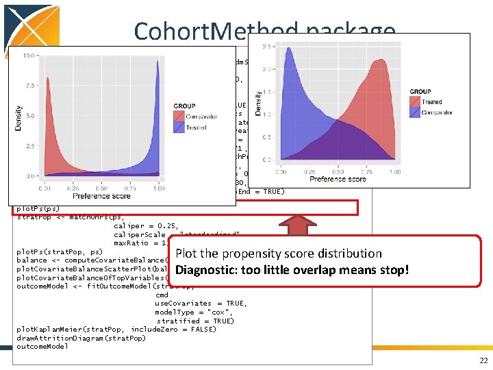
Cohort. Method package cmd <- get. Db. Cohort. Method. Data(connection. Details , cdm. Database. Schema = cdm. Schema, target. Id = 1118084, comparator. Id = 1124300, outcome. Id = 192671, washout. Period = 183, first. Exposure. Only = TRUE, remove. Duplicate. Subjects = TRUE, exclude. Drugs. From. Covariates = TRUE, covariate. Settings = create. Covariate. Settings()) study. Pop <- create. Study. Population(cohort. Method. Data = cmd, outcome. Id = 192671 , remove. Subjects. With. Prior. Outcome = TRUE, min. Days. At. Risk = 1, risk. Window. Start = 0, risk. Window. End = 30, add. Exposure. Days. To. End = TRUE) ps <- create. Ps(cmd, study. Pop) plot. Ps(ps) strat. Pop <- match. On. Ps(ps, caliper = 0. 25, caliper. Scale = "standardized", max. Ratio = 1) plot. Ps(strat. Pop, ps) balance <- compute. Covariate. Balance(strata, cmd) plot. Covariate. Balance. Scatter. Plot(balance) plot. Covariate. Balance. Of. Top. Variables(balance) outcome. Model <- fit. Outcome. Model(strat. Pop, cmd use. Covariates = TRUE, model. Type = "cox", stratified = TRUE) plot. Kaplan. Meier(strat. Pop, include. Zero = FALSE) draw. Attrition. Diagram(strat. Pop) outcome. Model Plot the propensity score distribution Diagnostic: too little overlap means stop! 22

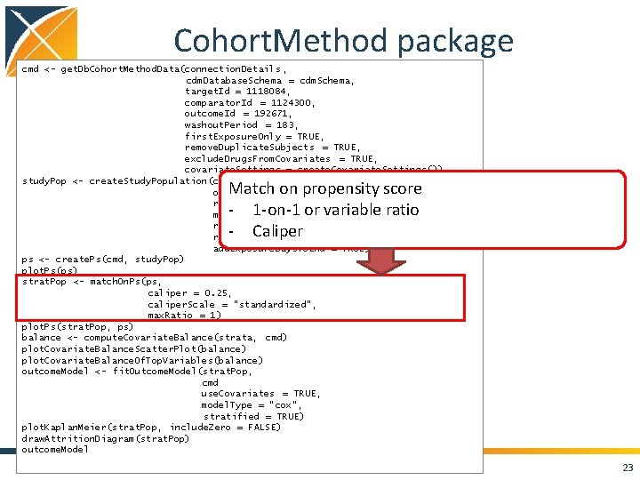
Cohort. Method package cmd <- get. Db. Cohort. Method. Data(connection. Details , cdm. Database. Schema = cdm. Schema, target. Id = 1118084, comparator. Id = 1124300, outcome. Id = 192671, washout. Period = 183, first. Exposure. Only = TRUE, remove. Duplicate. Subjects = TRUE, exclude. Drugs. From. Covariates = TRUE, covariate. Settings = create. Covariate. Settings()) study. Pop <- create. Study. Population(cohort. Method. Data = cmd, outcome. Id = 192671 , remove. Subjects. With. Prior. Outcome = TRUE, min. Days. At. Risk = 1, risk. Window. Start = 0, risk. Window. End = 30, add. Exposure. Days. To. End = TRUE) ps <- create. Ps(cmd, study. Pop) plot. Ps(ps) strat. Pop <- match. On. Ps(ps, caliper = 0. 25, caliper. Scale = "standardized", max. Ratio = 1) plot. Ps(strat. Pop, ps) balance <- compute. Covariate. Balance(strata, cmd) plot. Covariate. Balance. Scatter. Plot(balance) plot. Covariate. Balance. Of. Top. Variables(balance) outcome. Model <- fit. Outcome. Model(strat. Pop, cmd use. Covariates = TRUE, model. Type = "cox", stratified = TRUE) plot. Kaplan. Meier(strat. Pop, include. Zero = FALSE) draw. Attrition. Diagram(strat. Pop) outcome. Model Match on propensity score - 1 -on-1 or variable ratio - Caliper 23

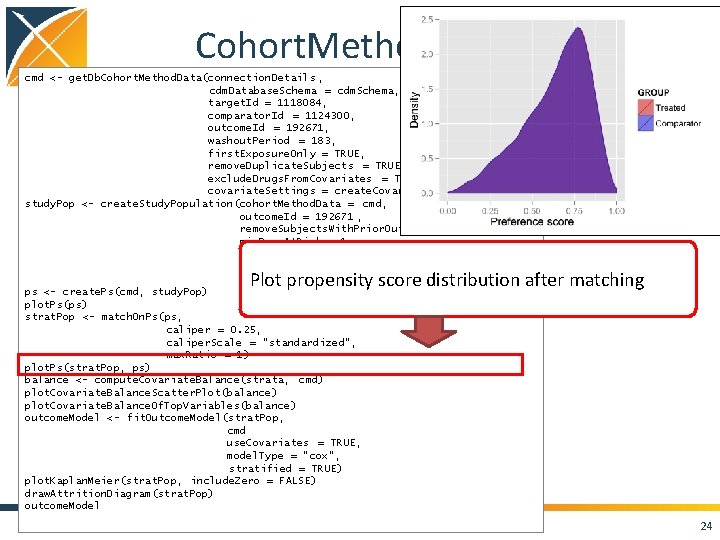
Cohort. Method package cmd <- get. Db. Cohort. Method. Data(connection. Details , cdm. Database. Schema = cdm. Schema, target. Id = 1118084, comparator. Id = 1124300, outcome. Id = 192671, washout. Period = 183, first. Exposure. Only = TRUE, remove. Duplicate. Subjects = TRUE, exclude. Drugs. From. Covariates = TRUE, covariate. Settings = create. Covariate. Settings()) study. Pop <- create. Study. Population(cohort. Method. Data = cmd, outcome. Id = 192671 , remove. Subjects. With. Prior. Outcome = TRUE, min. Days. At. Risk = 1, risk. Window. Start = 0, risk. Window. End = 30, add. Exposure. Days. To. End = TRUE) ps <- create. Ps(cmd, study. Pop) plot. Ps(ps) strat. Pop <- match. On. Ps(ps, caliper = 0. 25, caliper. Scale = "standardized", max. Ratio = 1) plot. Ps(strat. Pop, ps) balance <- compute. Covariate. Balance(strata, cmd) plot. Covariate. Balance. Scatter. Plot(balance) plot. Covariate. Balance. Of. Top. Variables(balance) outcome. Model <- fit. Outcome. Model(strat. Pop, cmd use. Covariates = TRUE, model. Type = "cox", stratified = TRUE) plot. Kaplan. Meier(strat. Pop, include. Zero = FALSE) draw. Attrition. Diagram(strat. Pop) outcome. Model Plot propensity score distribution after matching 24

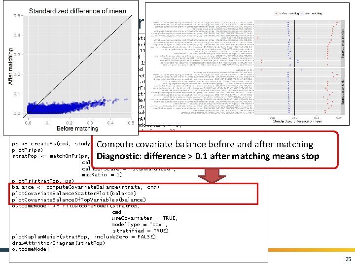
Cohort. Method package cmd <- get. Db. Cohort. Method. Data(connection. Details , cdm. Database. Schema = cdm. Schema, target. Id = 1118084, comparator. Id = 1124300, outcome. Id = 192671, washout. Period = 183, first. Exposure. Only = TRUE, remove. Duplicate. Subjects = TRUE, exclude. Drugs. From. Covariates = TRUE, covariate. Settings = create. Covariate. Settings()) study. Pop <- create. Study. Population(cohort. Method. Data = cmd, outcome. Id = 192671 , remove. Subjects. With. Prior. Outcome = TRUE, min. Days. At. Risk = 1, risk. Window. Start = 0, risk. Window. End = 30, add. Exposure. Days. To. End = TRUE) ps <- create. Ps(cmd, study. Pop) plot. Ps(ps) strat. Pop <- match. On. Ps(ps, caliper = 0. 25, caliper. Scale = "standardized", max. Ratio = 1) plot. Ps(strat. Pop, ps) balance <- compute. Covariate. Balance(strata, cmd) plot. Covariate. Balance. Scatter. Plot(balance) plot. Covariate. Balance. Of. Top. Variables(balance) outcome. Model <- fit. Outcome. Model(strat. Pop, cmd use. Covariates = TRUE, model. Type = "cox", stratified = TRUE) plot. Kaplan. Meier(strat. Pop, include. Zero = FALSE) draw. Attrition. Diagram(strat. Pop) outcome. Model Compute covariate balance before and after matching Diagnostic: difference > 0. 1 after matching means stop 25

Cohort. Method package cmd <- get. Db. Cohort. Method. Data(connection. Details , cdm. Database. Schema = cdm. Schema, target. Id = 1118084, comparator. Id = 1124300, outcome. Id = 192671, washout. Period = 183, first. Exposure. Only = TRUE, remove. Duplicate. Subjects = TRUE, exclude. Drugs. From. Covariates = TRUE, covariate. Settings = create. Covariate. Settings()) study. Pop <- create. Study. Population(cohort. Method. Data = cmd, outcome. Id = 192671 , remove. Subjects. With. Prior. Outcome = TRUE, min. Days. At. Risk = 1, risk. Window. Start = 0, risk. Window. End = 30, add. Exposure. Days. To. End = TRUE) ps <- create. Ps(cmd, study. Pop) plot. Ps(ps) strat. Pop <- match. On. Ps(ps, caliper = 0. 25, caliper. Scale = "standardized", max. Ratio = 1) plot. Ps(strat. Pop, ps) balance <- compute. Covariate. Balance(strata, cmd) plot. Covariate. Balance. Scatter. Plot(balance) plot. Covariate. Balance. Of. Top. Variables(balance) outcome. Model <- fit. Outcome. Model(strat. Pop, cmd use. Covariates = TRUE, model. Type = "cox", stratified = TRUE) plot. Kaplan. Meier(strat. Pop, include. Zero = FALSE) draw. Attrition. Diagram(strat. Pop) outcome. Model Fit the outcome model - Cox, Poisson, or logistic - Conditioned on matched sets / strata? - Include all covariates? 26

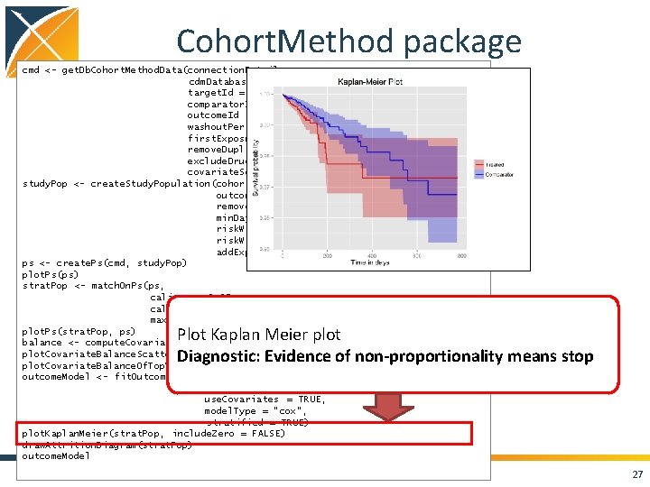
Cohort. Method package cmd <- get. Db. Cohort. Method. Data(connection. Details , cdm. Database. Schema = cdm. Schema, target. Id = 1118084, comparator. Id = 1124300, outcome. Id = 192671, washout. Period = 183, first. Exposure. Only = TRUE, remove. Duplicate. Subjects = TRUE, exclude. Drugs. From. Covariates = TRUE, covariate. Settings = create. Covariate. Settings()) study. Pop <- create. Study. Population(cohort. Method. Data = cmd, outcome. Id = 192671 , remove. Subjects. With. Prior. Outcome = TRUE, min. Days. At. Risk = 1, risk. Window. Start = 0, risk. Window. End = 30, add. Exposure. Days. To. End = TRUE) ps <- create. Ps(cmd, study. Pop) plot. Ps(ps) strat. Pop <- match. On. Ps(ps, caliper = 0. 25, caliper. Scale = "standardized", max. Ratio = 1) plot. Ps(strat. Pop, ps) balance <- compute. Covariate. Balance(strata, cmd) plot. Covariate. Balance. Scatter. Plot(balance) plot. Covariate. Balance. Of. Top. Variables(balance) outcome. Model <- fit. Outcome. Model(strat. Pop, cmd use. Covariates = TRUE, model. Type = "cox", stratified = TRUE) plot. Kaplan. Meier(strat. Pop, include. Zero = FALSE) draw. Attrition. Diagram(strat. Pop) outcome. Model Plot Kaplan Meier plot Diagnostic: Evidence of non-proportionality means stop 27

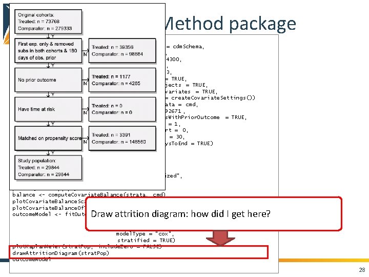
Cohort. Method package cmd <- get. Db. Cohort. Method. Data(connection. Details , cdm. Database. Schema = cdm. Schema, target. Id = 1118084, comparator. Id = 1124300, outcome. Id = 192671, washout. Period = 183, first. Exposure. Only = TRUE, remove. Duplicate. Subjects = TRUE, exclude. Drugs. From. Covariates = TRUE, covariate. Settings = create. Covariate. Settings()) study. Pop <- create. Study. Population(cohort. Method. Data = cmd, outcome. Id = 192671 , remove. Subjects. With. Prior. Outcome = TRUE, min. Days. At. Risk = 1, risk. Window. Start = 0, risk. Window. End = 30, add. Exposure. Days. To. End = TRUE) ps <- create. Ps(cmd, study. Pop) plot. Ps(ps) strat. Pop <- match. On. Ps(ps, caliper = 0. 25, caliper. Scale = "standardized", max. Ratio = 1) plot. Ps(strat. Pop, ps) balance <- compute. Covariate. Balance(strata, cmd) plot. Covariate. Balance. Scatter. Plot(balance) plot. Covariate. Balance. Of. Top. Variables(balance) outcome. Model <- fit. Outcome. Model(strat. Pop, cmd use. Covariates = TRUE, model. Type = "cox", stratified = TRUE) plot. Kaplan. Meier(strat. Pop, include. Zero = FALSE) draw. Attrition. Diagram(strat. Pop) outcome. Model Draw attrition diagram: how did I get here? 28

Cohort. Method package cmd <- get. Db. Cohort. Method. Data(connection. Details , cdm. Database. Schema = cdm. Schema, target. Id = 1118084, comparator. Id = 1124300, outcome. Id = 192671, washout. Period = 183, first. Exposure. Only = TRUE, remove. Duplicate. Subjects = TRUE, exclude. Drugs. From. Covariates = TRUE, covariate. Settings = create. Covariate. Settings()) study. Pop <- create. Study. Population(cohort. Method. Data = cmd, outcome. Id = 192671 , remove. Subjects. With. Prior. Outcome = TRUE, min. Days. At. Risk = 1, risk. Window. Start = 0, risk. Window. End = 30, add. Exposure. Days. To. End = TRUE) ps <- create. Ps(cmd, study. Pop) plot. Ps(ps) strat. Pop <- match. On. Ps(ps, caliper = 0. 25, caliper. Scale = "standardized", max. Ratio = 1) plot. Ps(strat. Pop, ps) balance <- compute. Covariate. Balance(strata, cmd) plot. Covariate. Balance. Scatter. Plot(balance) plot. Covariate. Balance. Of. Top. Variables(balance) outcome. Model <- fit. Outcome. Model(strat. Pop, cmd use. Covariates = TRUE, model. Type = "cox", stratified = TRUE) plot. Kaplan. Meier(strat. Pop, include. Zero = FALSE) draw. Attrition. Diagram(strat. Pop) outcome. Model Get outcome model 29

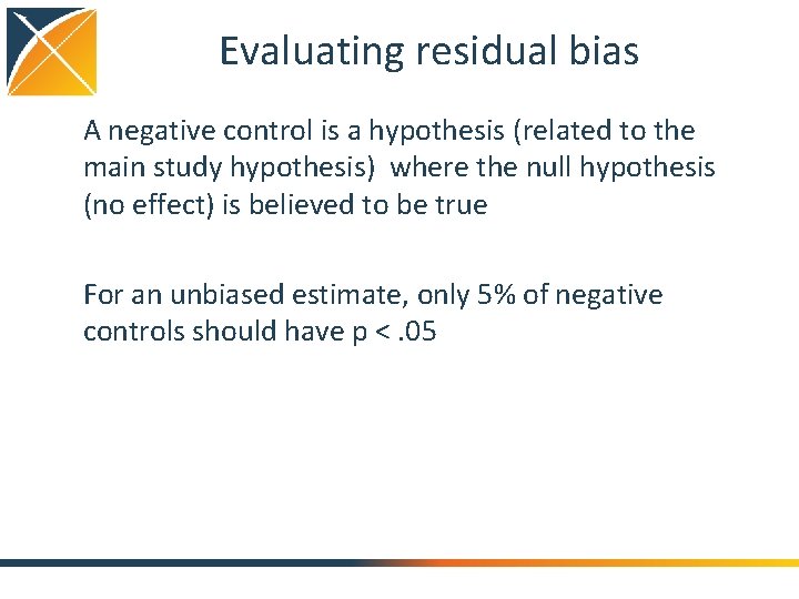
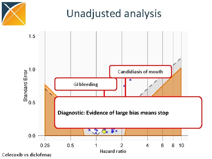
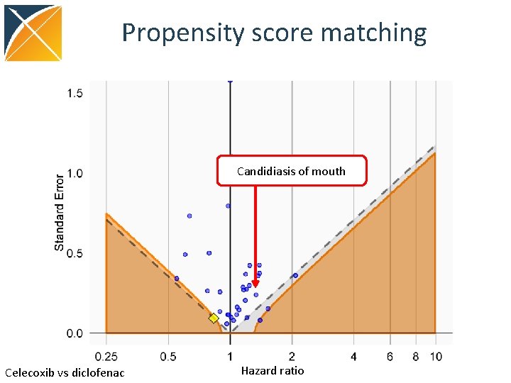
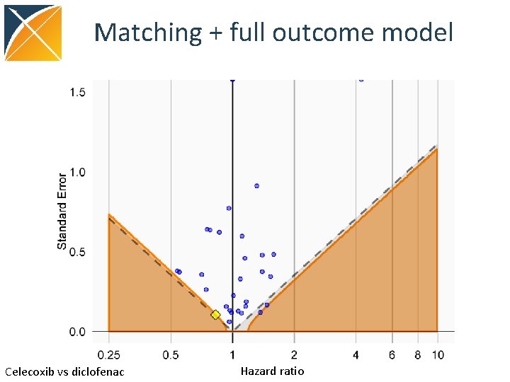
Evaluating residual bias A negative control is a hypothesis (related to the main study hypothesis) where the null hypothesis (no effect) is believed to be true For an unbiased estimate, only 5% of negative controls should have p <. 05

Unadjusted analysis Candidiasis of mouth GI bleeding Diagnostic: Evidence of large bias means stop Celecoxib vs diclofenac Hazard ratio

Propensity score matching Candidiasis of mouth Celecoxib vs diclofenac Hazard ratio

Matching + full outcome model Celecoxib vs diclofenac Hazard ratio

Conclusions • Cohort. Method package features – Large scale regression propensity models – Large scale regression outcome models • Using negative controls, we see a reduction in residual bias when using PS matching + full outcome model • We have already used Cohort. Method in several real studies

Next steps • Yuxi Tian (UCLA) is comparing our PS to HDPS • Need to write article showing ‘including instrumental variables in PS model leads to bias’ is nonsense • Disease risk scores instead of PS? • Inverse probability weighting?

Topic of next meeting(s)? • Method evaluation • Identifying the important questions that can be answered using observational research • Replicating RCTs in observational data • TMU’s web-based case-control study app • ? 36

Next workgroup meeting May 18 • 3 pm Hong Kong / Taiwan • 4 pm South Korea • 4: 30 pm Adelaide • 9 am Central European time http: //www. ohdsi. org/web/wiki/doku. php? id=projects: workgroups: est-methods 37