Appendix A FIGURE A 2 1 Historical PC
- Slides: 40

Appendix A

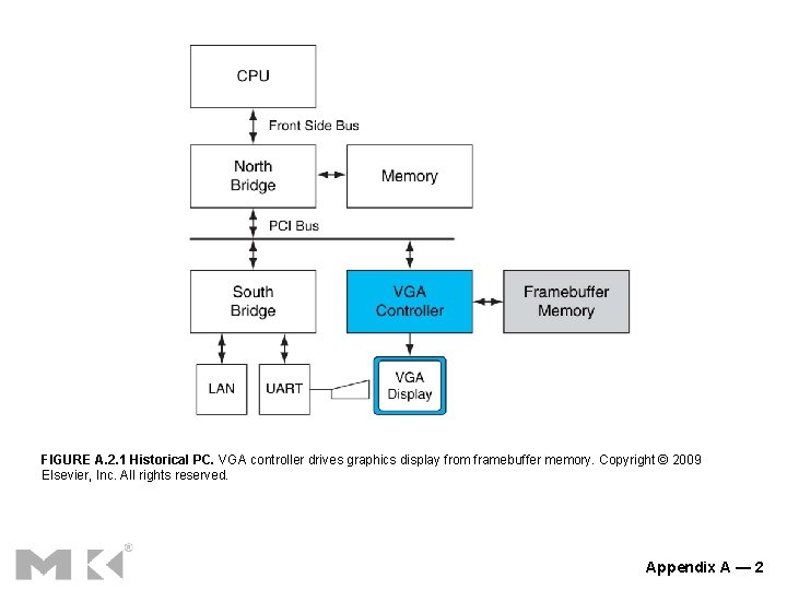
FIGURE A. 2. 1 Historical PC. VGA controller drives graphics display from framebuffer memory. Copyright © 2009 Elsevier, Inc. All rights reserved. Appendix A — 2

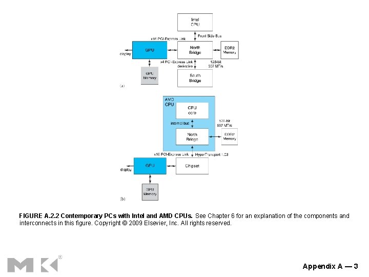
FIGURE A. 2. 2 Contemporary PCs with Intel and AMD CPUs. See Chapter 6 for an explanation of the components and interconnects in this figure. Copyright © 2009 Elsevier, Inc. All rights reserved. Appendix A — 3

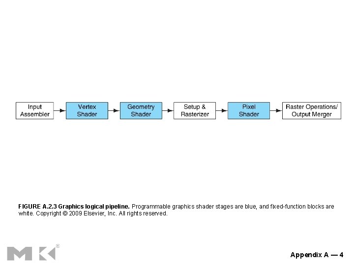
FIGURE A. 2. 3 Graphics logical pipeline. Programmable graphics shader stages are blue, and fixed-function blocks are white. Copyright © 2009 Elsevier, Inc. All rights reserved. Appendix A — 4

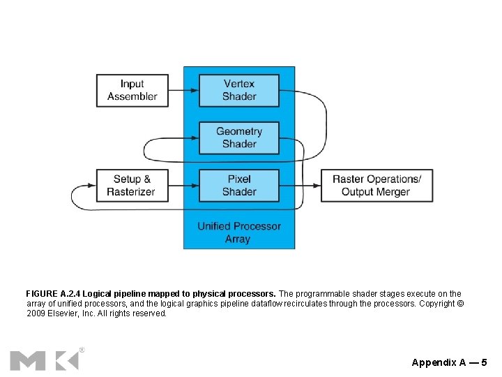
FIGURE A. 2. 4 Logical pipeline mapped to physical processors. The programmable shader stages execute on the array of unified processors, and the logical graphics pipeline dataflow recirculates through the processors. Copyright © 2009 Elsevier, Inc. All rights reserved. Appendix A — 5

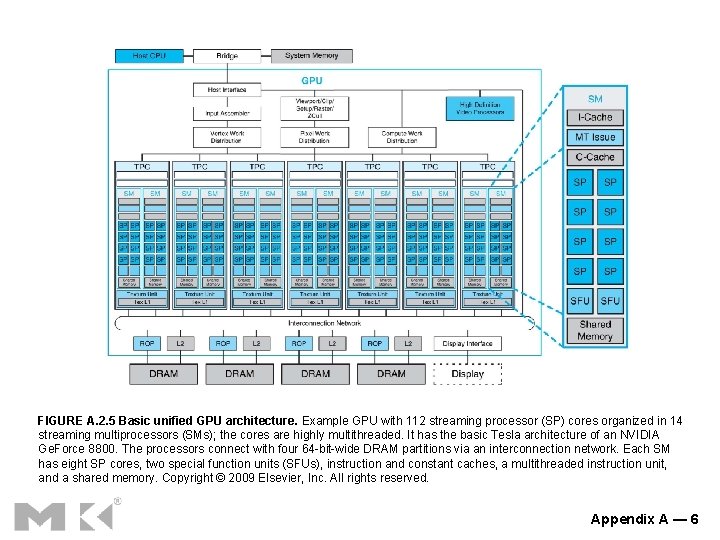
FIGURE A. 2. 5 Basic unified GPU architecture. Example GPU with 112 streaming processor (SP) cores organized in 14 streaming multiprocessors (SMs); the cores are highly multithreaded. It has the basic Tesla architecture of an NVIDIA Ge. Force 8800. The processors connect with four 64 -bit-wide DRAM partitions via an interconnection network. Each SM has eight SP cores, two special function units (SFUs), instruction and constant caches, a multithreaded instruction unit, and a shared memory. Copyright © 2009 Elsevier, Inc. All rights reserved. Appendix A — 6

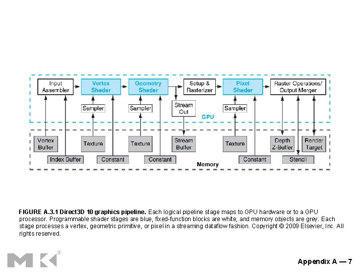
FIGURE A. 3. 1 Direct 3 D 10 graphics pipeline. Each logical pipeline stage maps to GPU hardware or to a GPU processor. Programmable shader stages are blue, fixed-function blocks are white, and memory objects are grey. Each stage processes a vertex, geometric primitive, or pixel in a streaming dataflow fashion. Copyright © 2009 Elsevier, Inc. All rights reserved. Appendix A — 7

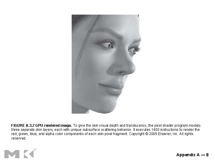
FIGURE A. 3. 2 GPU-rendered image. To give the skin visual depth and translucency, the pixel shader program models three separate skin layers, each with unique subsurface scattering behavior. It executes 1400 instructions to render the red, green, blue, and alpha color components of each skin pixel fragment. Copyright © 2009 Elsevier, Inc. All rights reserved. Appendix A — 8

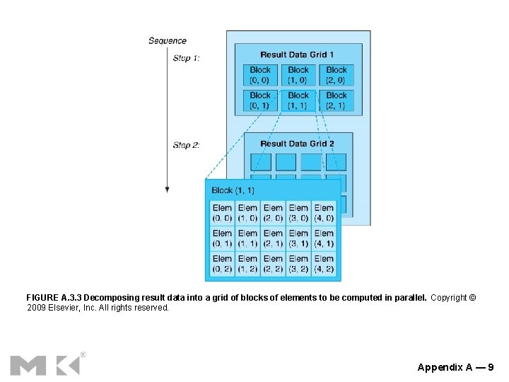
FIGURE A. 3. 3 Decomposing result data into a grid of blocks of elements to be computed in parallel. Copyright © 2009 Elsevier, Inc. All rights reserved. Appendix A — 9

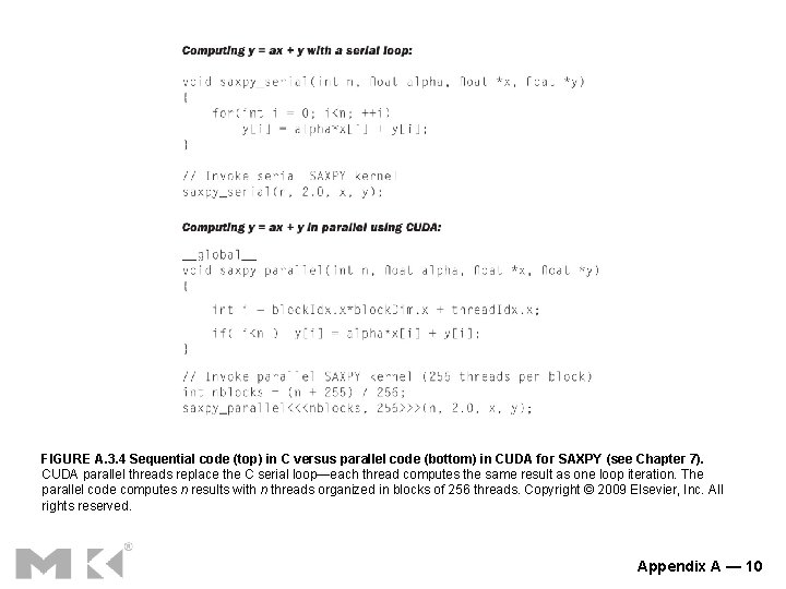
FIGURE A. 3. 4 Sequential code (top) in C versus parallel code (bottom) in CUDA for SAXPY (see Chapter 7). CUDA parallel threads replace the C serial loop—each thread computes the same result as one loop iteration. The parallel code computes n results with n threads organized in blocks of 256 threads. Copyright © 2009 Elsevier, Inc. All rights reserved. Appendix A — 10

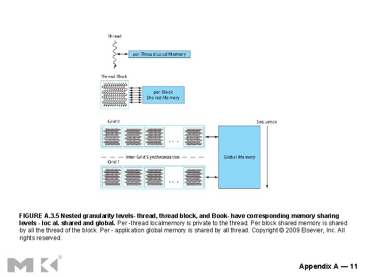
FIGURE A. 3. 5 Nested granularity levels- thread, thread block, and Book- have corresponding memory sharing levels - loc al. shared and global. Per -thread localmemory is private to the thread. Per block shared memory is shared by all the thread of the block. Per - application global memory is shared by all thread. Copyright © 2009 Elsevier, Inc. All rights reserved. Appendix A — 11

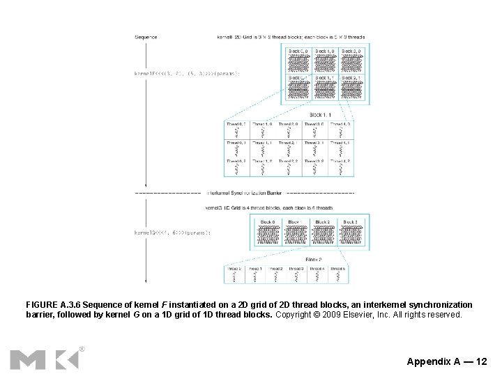
FIGURE A. 3. 6 Sequence of kernel F instantiated on a 2 D grid of 2 D thread blocks, an interkernel synchronization barrier, followed by kernel G on a 1 D grid of 1 D thread blocks. Copyright © 2009 Elsevier, Inc. All rights reserved. Appendix A — 12

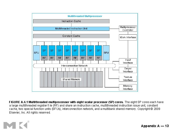
FIGURE A. 4. 1 Multithreaded multiprocessor with eight scalar processor (SP) cores. The eight SP cores each have a large multithreaded register fi le (RF) and share an instruction cache, multithreaded instruction issue unit, constant cache, two special function units (SFUs), interconnection network, and a multibank shared memory. Copyright © 2009 Elsevier, Inc. All rights reserved. Appendix A — 13

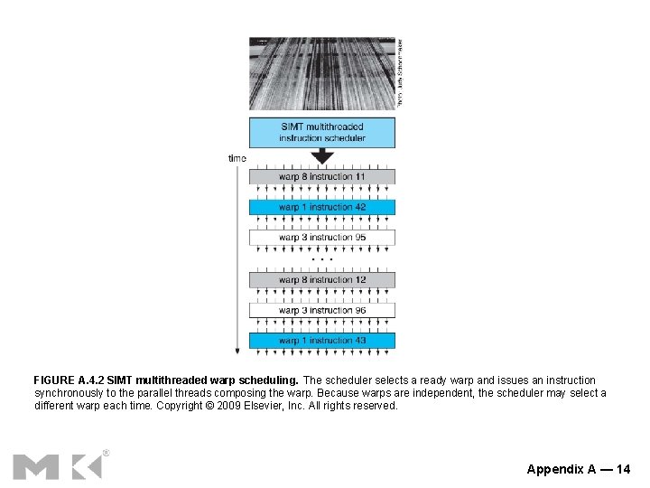
FIGURE A. 4. 2 SIMT multithreaded warp scheduling. The scheduler selects a ready warp and issues an instruction synchronously to the parallel threads composing the warp. Because warps are independent, the scheduler may select a different warp each time. Copyright © 2009 Elsevier, Inc. All rights reserved. Appendix A — 14

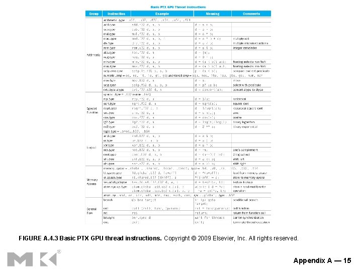
FIGURE A. 4. 3 Basic PTX GPU thread instructions. Copyright © 2009 Elsevier, Inc. All rights reserved. Appendix A — 15

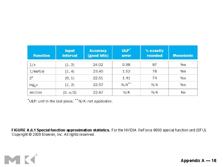
FIGURE A. 6. 1 Special function approximation statistics. For the NVIDIA Ge. Force 8800 special function unit (SFU). Copyright © 2009 Elsevier, Inc. All rights reserved. Appendix A — 16

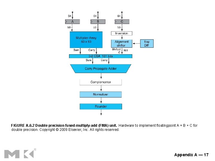
FIGURE A. 6. 2 Double precision fused-multiply-add (FMA) unit. Hardware to implement floatingpoint A × B + C for double precision. Copyright © 2009 Elsevier, Inc. All rights reserved. Appendix A — 17

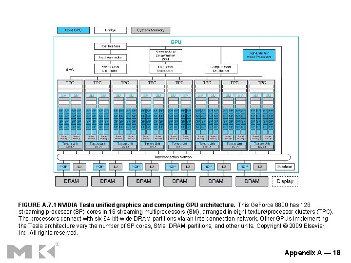
FIGURE A. 7. 1 NVIDIA Tesla unified graphics and computing GPU architecture. This Ge. Force 8800 has 128 streaming processor (SP) cores in 16 streaming multiprocessors (SM), arranged in eight texture/processor clusters (TPC). The processors connect with six 64 -bit-wide DRAM partitions via an interconnection network. Other GPUs implementing the Tesla architecture vary the number of SP cores, SMs, DRAM partitions, and other units. Copyright © 2009 Elsevier, Inc. All rights reserved. Appendix A — 18

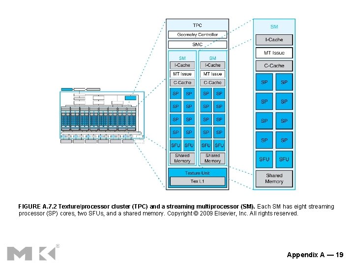
FIGURE A. 7. 2 Texture/processor cluster (TPC) and a streaming multiprocessor (SM). Each SM has eight streaming processor (SP) cores, two SFUs, and a shared memory. Copyright © 2009 Elsevier, Inc. All rights reserved. Appendix A — 19

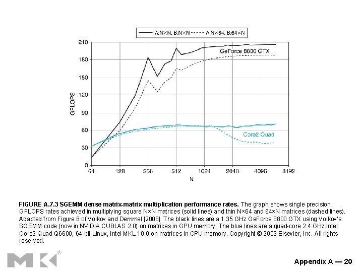
FIGURE A. 7. 3 SGEMM dense matrix-matrix multiplication performance rates. The graph shows single precision GFLOPS rates achieved in multiplying square N×N matrices (solid lines) and thin N× 64 and 64×N matrices (dashed lines). Adapted from Figure 6 of Volkov and Demmel [2008]. The black lines are a 1. 35 GHz Ge. Force 8800 GTX using Volkov’s SGEMM code (now in NVIDIA CUBLAS 2. 0) on matrices in GPU memory. The blue lines are a quad-core 2. 4 GHz Intel Core 2 Quad Q 6600, 64 -bit Linux, Intel MKL 10. 0 on matrices in CPU memory. Copyright © 2009 Elsevier, Inc. All rights reserved. Appendix A — 20

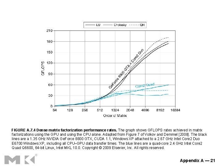
FIGURE A. 7. 4 Dense matrix factorization performance rates. The graph shows GFLOPS rates achieved in matrix factorizations using the GPU and using the CPU alone. Adapted from Figure 7 of Volkov and Demmel [2008]. The black lines are a 1. 35 GHz NVIDIA Ge. Force 8800 GTX, CUDA 1. 1, Windows XP attached to a 2. 67 GHz Intel Core 2 Duo E 6700 Windows XP, including all CPU–GPU data transfer times. The blue lines are a quad-core 2. 4 GHz Intel Core 2 Quad Q 6600, 64 -bit Linux, Intel MKL 10. 0. Copyright © 2009 Elsevier, Inc. All rights reserved. Appendix A — 21

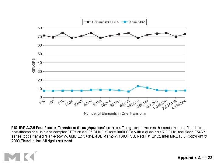
FIGURE A. 7. 5 Fast Fourier Transform throughput performance. The graph compares the performance of batched one-dimensional in-place complex FFTs on a 1. 35 GHz Ge. Force 8800 GTX with a quad-core 2. 8 GHz Intel Xeon E 5462 series (code named “Harpertown”), 6 MB L 2 Cache, 4 GB Memory, 1600 FSB, Red Hat Linux, Intel MKL 10. 0. Copyright © 2009 Elsevier, Inc. All rights reserved. Appendix A — 22

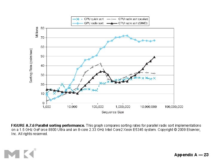
FIGURE A. 7. 6 Parallel sorting performance. This graph compares sorting rates for parallel radix sort implementations on a 1. 5 GHz Ge. Force 8800 Ultra and an 8 -core 2. 33 GHz Intel Core 2 Xeon E 5345 system. Copyright © 2009 Elsevier, Inc. All rights reserved. Appendix A — 23

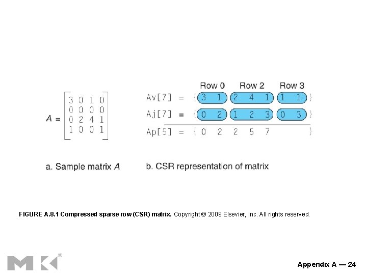
FIGURE A. 8. 1 Compressed sparse row (CSR) matrix. Copyright © 2009 Elsevier, Inc. All rights reserved. Appendix A — 24

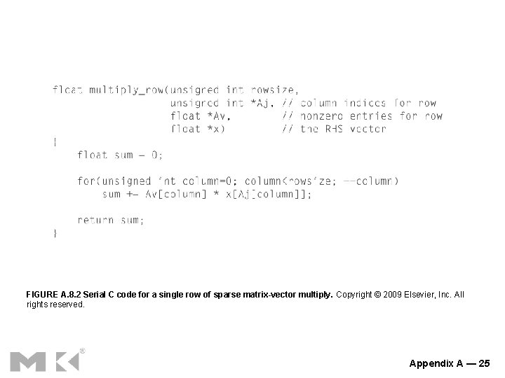
FIGURE A. 8. 2 Serial C code for a single row of sparse matrix-vector multiply. Copyright © 2009 Elsevier, Inc. All rights reserved. Appendix A — 25

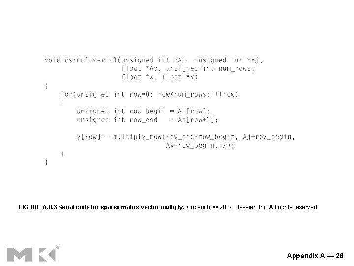
FIGURE A. 8. 3 Serial code for sparse matrix-vector multiply. Copyright © 2009 Elsevier, Inc. All rights reserved. Appendix A — 26

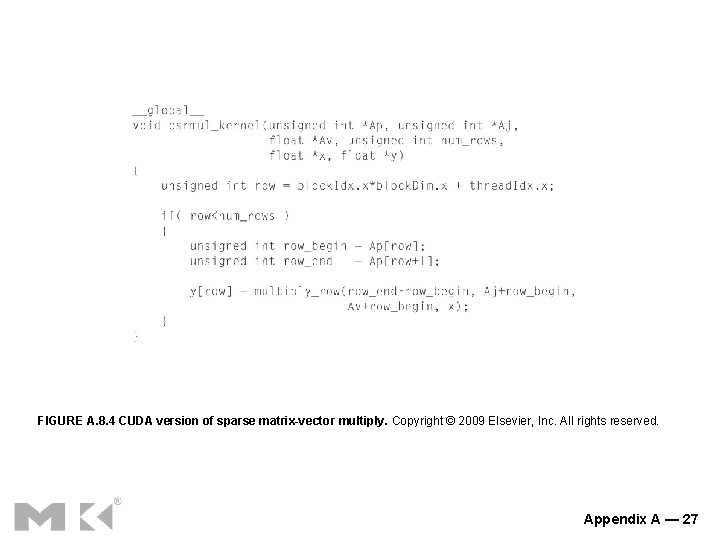
FIGURE A. 8. 4 CUDA version of sparse matrix-vector multiply. Copyright © 2009 Elsevier, Inc. All rights reserved. Appendix A — 27

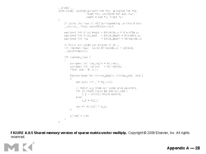
FIGURE A. 8. 5 Shared memory version of sparse matrix-vector multiply. Copyright © 2009 Elsevier, Inc. All rights reserved. Appendix A — 28

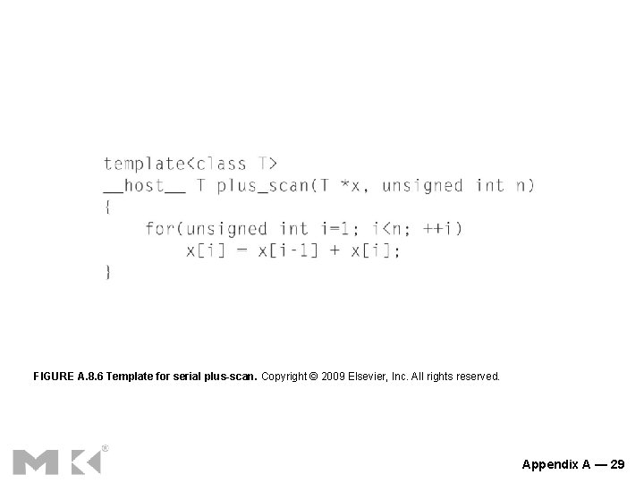
FIGURE A. 8. 6 Template for serial plus-scan. Copyright © 2009 Elsevier, Inc. All rights reserved. Appendix A — 29

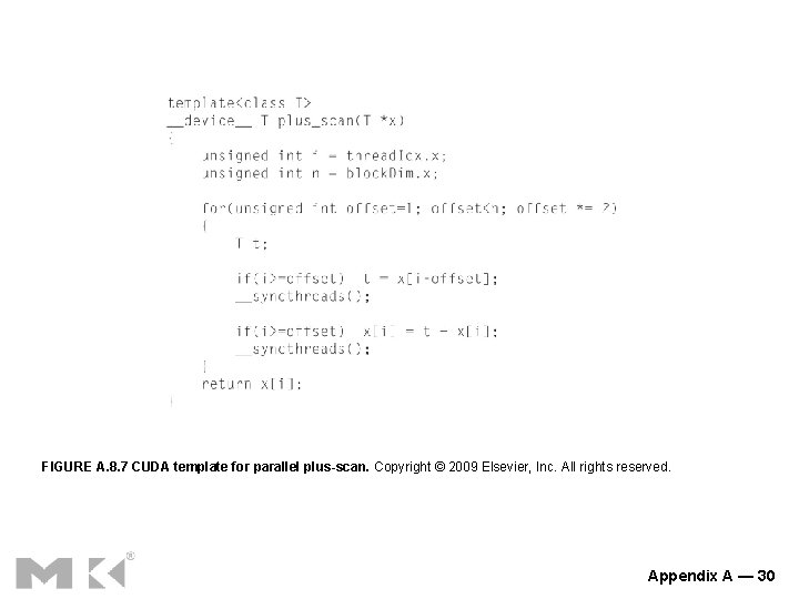
FIGURE A. 8. 7 CUDA template for parallel plus-scan. Copyright © 2009 Elsevier, Inc. All rights reserved. Appendix A — 30

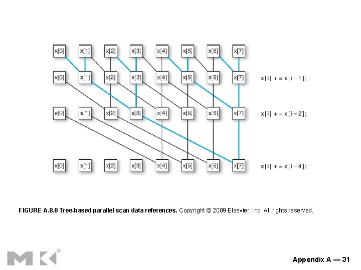
FIGURE A. 8. 8 Tree-based parallel scan data references. Copyright © 2009 Elsevier, Inc. All rights reserved. Appendix A — 31

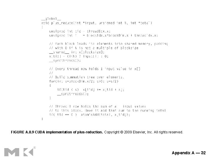
FIGURE A. 8. 9 CUDA implementation of plus-reduction. Copyright © 2009 Elsevier, Inc. All rights reserved. Appendix A — 32

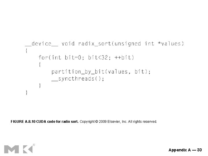
FIGURE A. 8. 10 CUDA code for radix sort. Copyright © 2009 Elsevier, Inc. All rights reserved. Appendix A — 33

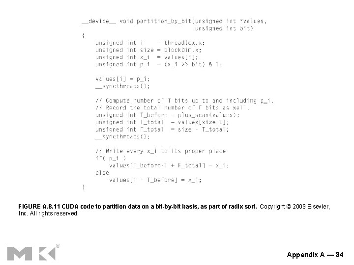
FIGURE A. 8. 11 CUDA code to partition data on a bit-by-bit basis, as part of radix sort. Copyright © 2009 Elsevier, Inc. All rights reserved. Appendix A — 34

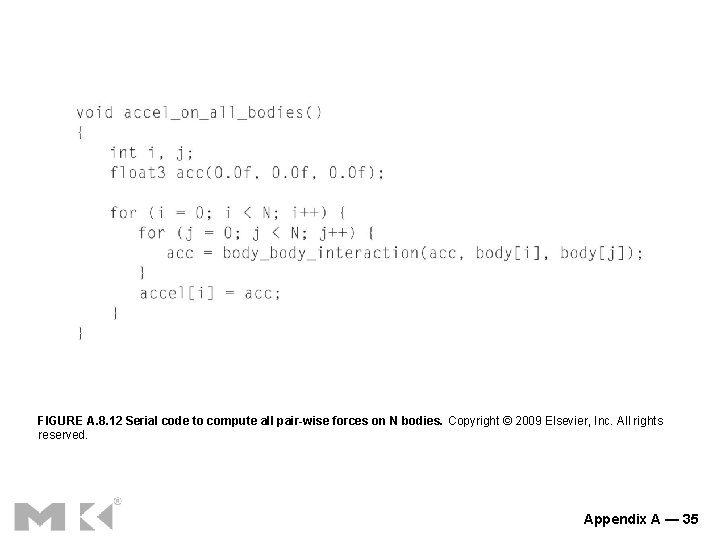
FIGURE A. 8. 12 Serial code to compute all pair-wise forces on N bodies. Copyright © 2009 Elsevier, Inc. All rights reserved. Appendix A — 35

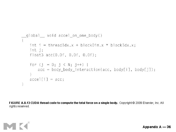
FIGURE A. 8. 13 CUDA thread code to compute the total force on a single body. Copyright © 2009 Elsevier, Inc. All rights reserved. Appendix A — 36

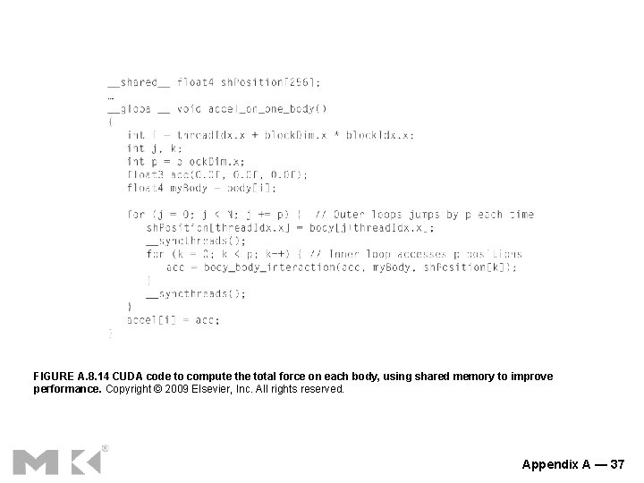
FIGURE A. 8. 14 CUDA code to compute the total force on each body, using shared memory to improve performance. Copyright © 2009 Elsevier, Inc. All rights reserved. Appendix A — 37

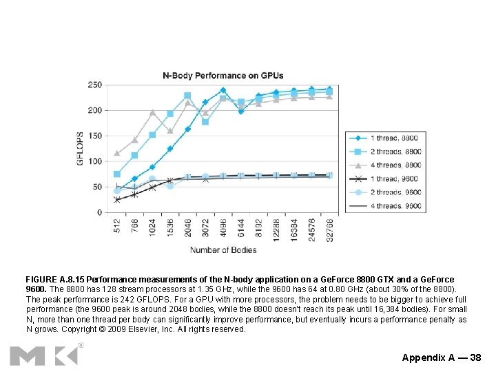
FIGURE A. 8. 15 Performance measurements of the N-body application on a Ge. Force 8800 GTX and a Ge. Force 9600. The 8800 has 128 stream processors at 1. 35 GHz, while the 9600 has 64 at 0. 80 GHz (about 30% of the 8800). The peak performance is 242 GFLOPS. For a GPU with more processors, the problem needs to be bigger to achieve full performance (the 9600 peak is around 2048 bodies, while the 8800 doesn’t reach its peak until 16, 384 bodies). For small N, more than one thread per body can significantly improve performance, but eventually incurs a performance penalty as N grows. Copyright © 2009 Elsevier, Inc. All rights reserved. Appendix A — 38

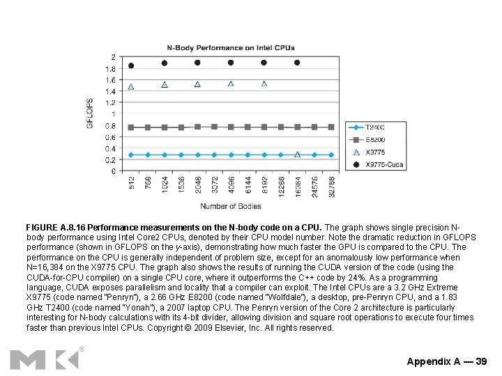
FIGURE A. 8. 16 Performance measurements on the N-body code on a CPU. The graph shows single precision Nbody performance using Intel Core 2 CPUs, denoted by their CPU model number. Note the dramatic reduction in GFLOPS performance (shown in GFLOPS on the y-axis), demonstrating how much faster the GPU is compared to the CPU. The performance on the CPU is generally independent of problem size, except for an anomalously low performance when N=16, 384 on the X 9775 CPU. The graph also shows the results of running the CUDA version of the code (using the CUDA-for-CPU compiler) on a single CPU core, where it outperforms the C++ code by 24%. As a programming language, CUDA exposes parallelism and locality that a compiler can exploit. The Intel CPUs are a 3. 2 GHz Extreme X 9775 (code named “Penryn”), a 2. 66 GHz E 8200 (code named “Wolfdale”), a desktop, pre-Penryn CPU, and a 1. 83 GHz T 2400 (code named “Yonah”), a 2007 laptop CPU. The Penryn version of the Core 2 architecture is particularly interesting for N-body calculations with its 4 -bit divider, allowing division and square root operations to execute four times faster than previous Intel CPUs. Copyright © 2009 Elsevier, Inc. All rights reserved. Appendix A — 39

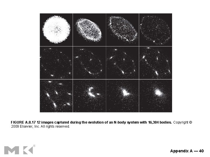
FIGURE A. 8. 17 12 images captured during the evolution of an N-body system with 16, 384 bodies. Copyright © 2009 Elsevier, Inc. All rights reserved. Appendix A — 40