Appendix A Fourier transform Appendix Linear systems Appendix

Appendix A : Fourier transform

Appendix : Linear systems

Appendix : Shift-invariant systems

Impulse-response function : h(t) Transfer function : H(n) Impulse-response function (the response of the system to an impulse, or a point, at the input) Transfer function (the response to spatial harmonic functions)

Appendix : Transfer function

4. Fourier Optics

2 D Fourier transform Plane wave In a plane (e. g. z=0) (harmonic function) One-to-one correspondence because with “+”, forward “-” , backward

In general (superposition integral of harmonic functions) The transmitted wave is a superposition of plane wave Superposition of plane waves

Spatial harmonic function and plane wave

Spatial spectral analysis

Spatial frequency and propagation angle

Amplitude modulation

B. Transfer Function of Free Space Impulse response function h Transfer function H

Transfer Function of Free Space : evanescent wave We may therefore regard 1/l as the cutoff spatial frequency (the spatial bandwidth) of the system

Fresnel approximation for transfer function of free space If a is the largest radial distance in the output plane, the largest angle qm a/d, and we may write

Input - Output Relation

Impulse-Response Function of Free Space = Inverse Fourier transform of the transfer function Paraboloidal wave Free-Space Propagation as a Convolution

Huygens-Fresnel Principle and the impulse-response function The Huygens-Fresnel principle states that each point on a wavefront generates a spherical wave. The envelope of these secondary waves constitutes a new wavefront. Their superposition constitutes the wave in another plane. The system’s impulse-response function for propagation between the planes z = 0 and z = d is In the paraxial approximation, the spherical wave is approximated by the paraboloidal wave. Our derivation of the impulse response function is therefore consistent with the H. -F. principle.

In summary: Within the Fresnel approximation, there are two approaches to determining the complex amplitude g(x, y) in the output plane, given the complex amplitude f(x, y) in the input plane: Space-domain approach in which the input wave is expanded in terms of paraboloidal elementary waves Frequency-domain approach in which the input wave is expanded as a sum of plane waves.

4. 2 Optical Fourier transform A. Fourier Transform in the Far Field If the propagation distance d is sufficiently long, the only plane wave that contributes to the complex amplitude at a point (x, y) in the output plane is the wave with direction making angles Proof!

Proof : for Fraunhofer approximation If f(x, y) is confined to a small area of radius b, and if the distance d is sufficiently large so that the Fresnel number is small, Condition of Validity of Fraunhofer Approximation when the Fresnel number

Three configurations back focal plane Input placed against lens Input placed in front of lens Input placed behind lens Phase representation of a thin lens in paraxial approximation

(a) The input placed directly against the lens Pupil function ; Ul From the Fresnel approximation when d = f , Quadratic phase factor Fourier transform Ul’

(b) The input placed in front of the lens If d = f Exact Fourier transform !

(c) The input placed behind the lens Scaleable Fourier transform ! As d reduces, the scale of the transform is made smaller.

In summary, convex lens can perform Fourier transformation The intensity at the back focal plane of the lens is therefore proportional to the squared absolute value of the Fourier transform of the complex amplitude of the wave at the input plane, regardless of the distance d.

4. 3 Regimes of Diffraction of Light

A. Fraunhofer diffraction Aperture function : d b

Note, for focusing Gaussian beam with an infinitely large lens, Radius :

B. Fresnel diffraction

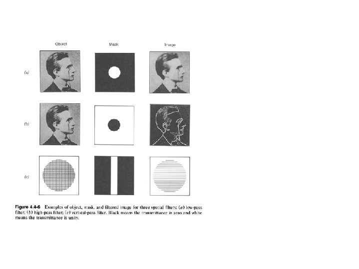
Spatial filtering in 4 -f system

Transfer Function of the 4 -f Spatial Filter With Mask Transmittance p(x, y) : The transfer function has the same shape as the pupil function. Impulse-response function is

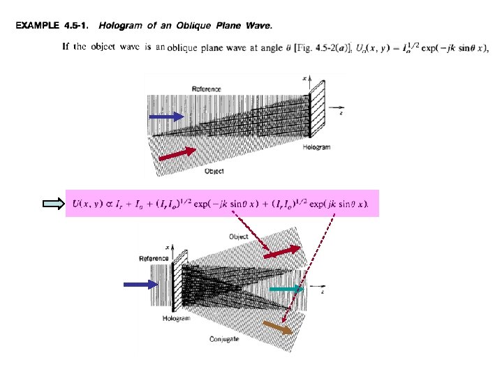
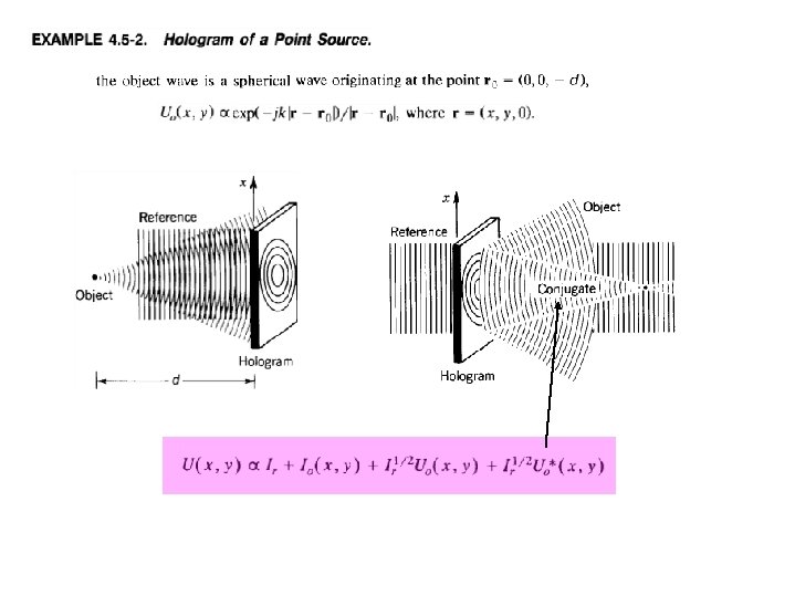
4. 5 Holography If the reference wave is a uniform plane wave, Original object wave!!

Off-axis holography ( qmin qs/2 ) 2 qs Spreading-angle width : qs Assume that the object wave has a complex amplitude Ambiguity term

Fourier-transform holography

Holographic spatial filters IFT Called “ Vander Lugt filter” or “Vander Lugt correlator”

Volume holography THICK Recording medium Transmission hologram : Reflection hologram :

Volume holographic grating kg Grating vector kr kg = k 0 - k r k 0 Grating period L = 2 p/ |kg| Proof !!

Volume holographic grating = Bragg grating Bragg condition :

“Holographic data storage prepares for the real world” Laser Focus World – October 2003 200 -Gbyte capacity in disk form factor 100 Mbyte/s data-transfer rate “Holographic storage drives such as this prototype from Aprilis are expected to become commercially available for write-once-read-many (WORM) applications in 2005. ”

C. Single-lens imaging system Impulse response function At the aperture plane : Beyond the lens : Assume d 1 = f

Single-lens imaging system Transfer function

Imaging property of a convex lens From an input point S to the output point P ; magnification Fig. 1. 22, Iizuka

Diffraction-limited imaging of a convex lens From a finite-sized square aperture of dimension a x a to near the output point P ;