Analysis of Covariance ANCOVA GLM 2 Prof Andy

Analysis of Covariance, ANCOVA (GLM 2) Prof. Andy Field Slide 1

Aims • • When and why do we use ANCOVA? Partitioning Variance Carrying out on IBM SPSS Interpretation – Main Effects – Covariates Slide

When And Why • To test for differences between group means when we know that an extraneous variable affects the outcome variable. • Used to held known extraneous variables constant. Slide

Advantages of ANCOVA • Reduces Error Variance – By explaining some of the unexplained variance (SSR) the error variance in the model can be reduced. • Greater Experimental Control: – By holding known extraneous variables constant, we gain greater insight into the effect of the predictor variable(s). Slide

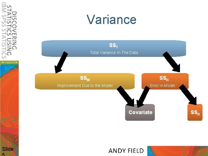
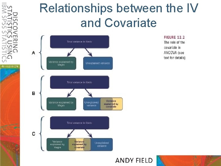
Variance SST Total Variance In The Data SSM Improvement Due to the Model SSR Error in Model Covariate Slide SSR

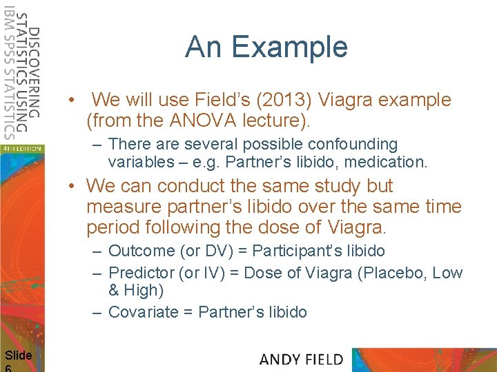
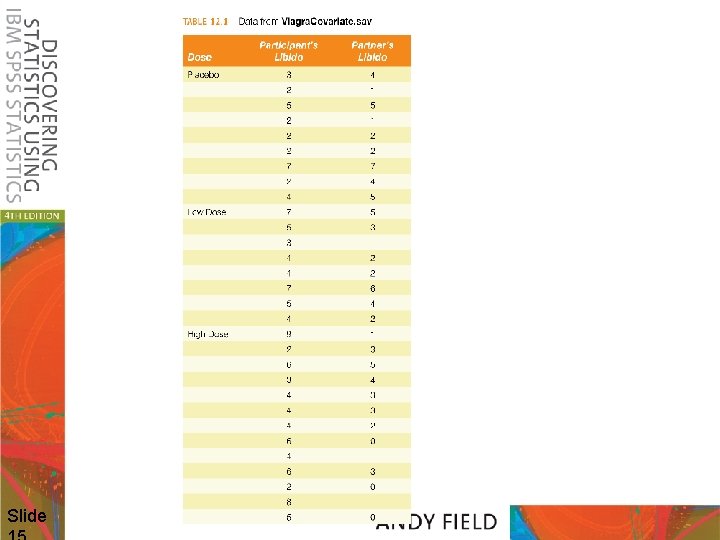
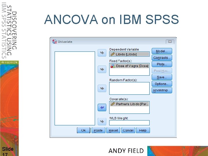
An Example • We will use Field’s (2013) Viagra example (from the ANOVA lecture). – There are several possible confounding variables – e. g. Partner’s libido, medication. • We can conduct the same study but measure partner’s libido over the same time period following the dose of Viagra. – Outcome (or DV) = Participant’s libido – Predictor (or IV) = Dose of Viagra (Placebo, Low & High) – Covariate = Partner’s libido Slide

Relationships between the IV and Covariate

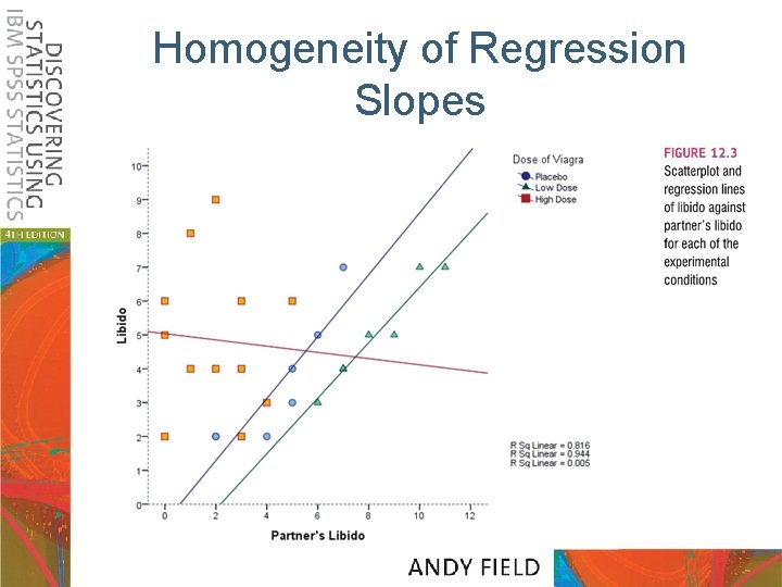
Homogeneity of Regression Slopes

Slide

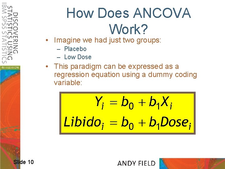
How Does ANCOVA Work? • Imagine we had just two groups: – Placebo – Low Dose • This paradigm can be expressed as a regression equation using a dummy coding variable: Slide 10

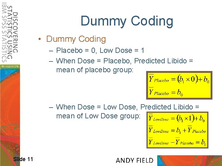
Dummy Coding • Dummy Coding – Placebo = 0, Low Dose = 1 – When Dose = Placebo, Predicted Libido = mean of placebo group: – When Dose = Low Dose, Predicted Libido = mean of Low Dose group: Slide 11

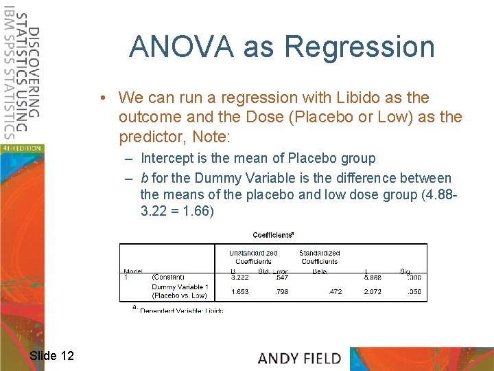
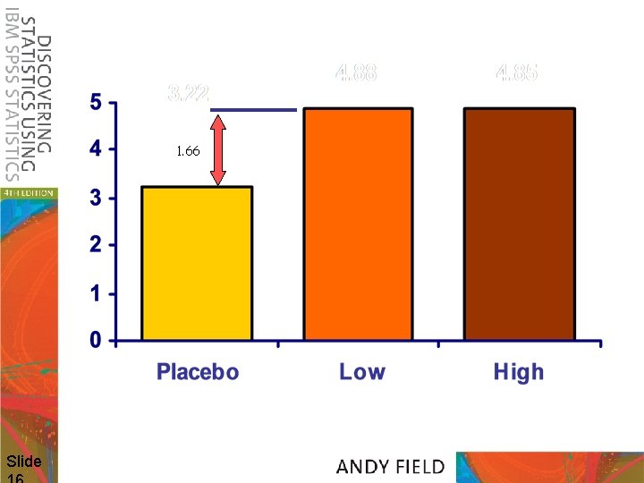
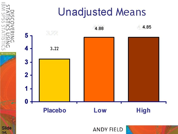
ANOVA as Regression • We can run a regression with Libido as the outcome and the Dose (Placebo or Low) as the predictor, Note: – Intercept is the mean of Placebo group – b for the Dummy Variable is the difference between the means of the placebo and low dose group (4. 883. 22 = 1. 66) Slide 12

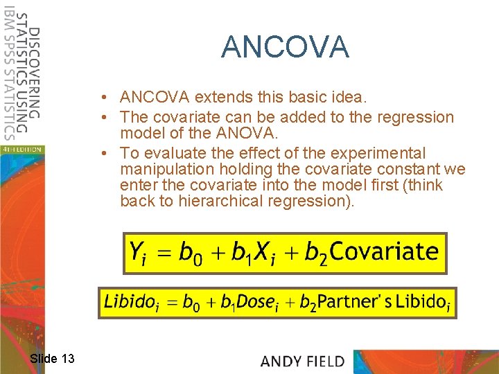
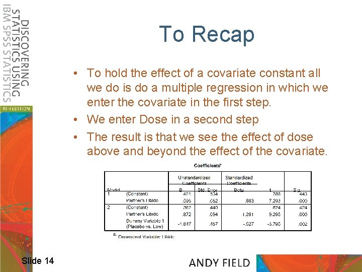
ANCOVA • ANCOVA extends this basic idea. • The covariate can be added to the regression model of the ANOVA. • To evaluate the effect of the experimental manipulation holding the covariate constant we enter the covariate into the model first (think back to hierarchical regression). Slide 13

To Recap • To hold the effect of a covariate constant all we do is do a multiple regression in which we enter the covariate in the first step. • We enter Dose in a second step • The result is that we see the effect of dose above and beyond the effect of the covariate. Slide 14

Slide

1. 66 Slide

ANCOVA on IBM SPSS Slide

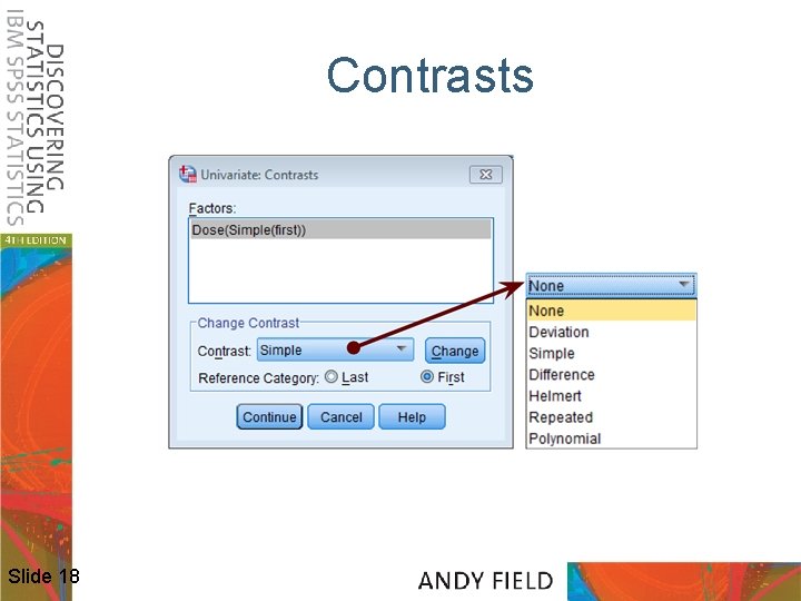
Contrasts Slide 18

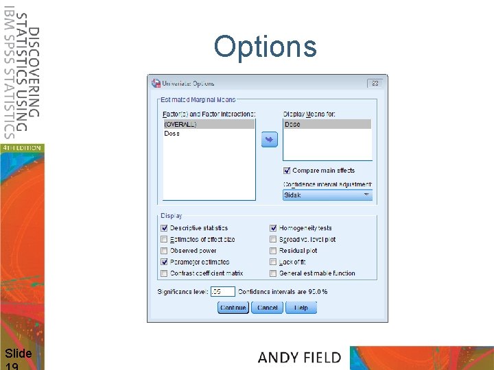
Options Slide

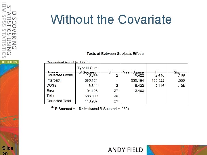
Without the Covariate Slide

Output Slide

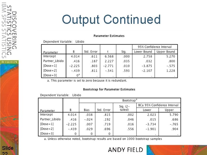
Output Continued Slide

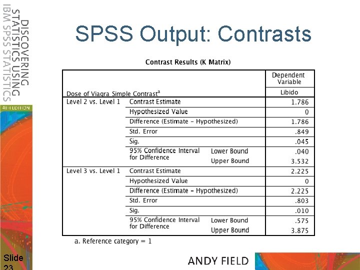
SPSS Output: Contrasts Slide

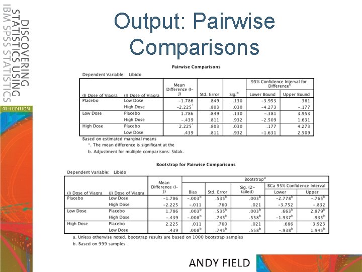
Output: Pairwise Comparisons

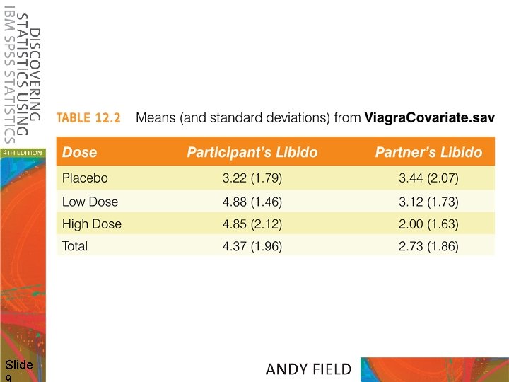
Unadjusted Means 4. 88 3. 22 Slide 4. 85

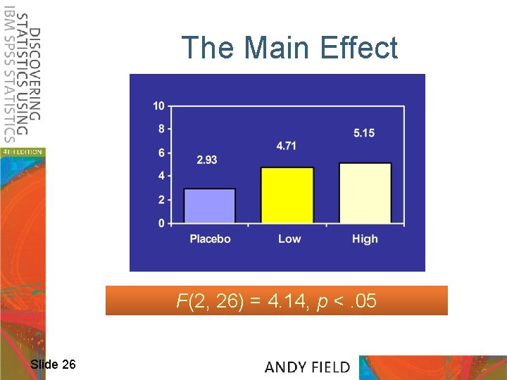
The Main Effect F(2, 26) = 4. 14, p <. 05 Slide 26

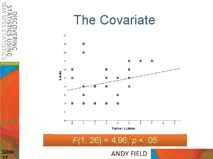
The Covariate F(1, 26) = 4. 96, p <. 05 Slide

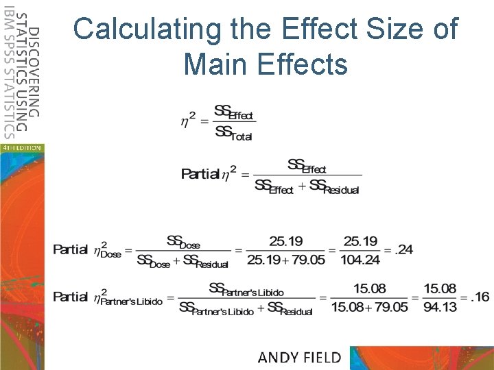
Calculating the Effect Size of Main Effects

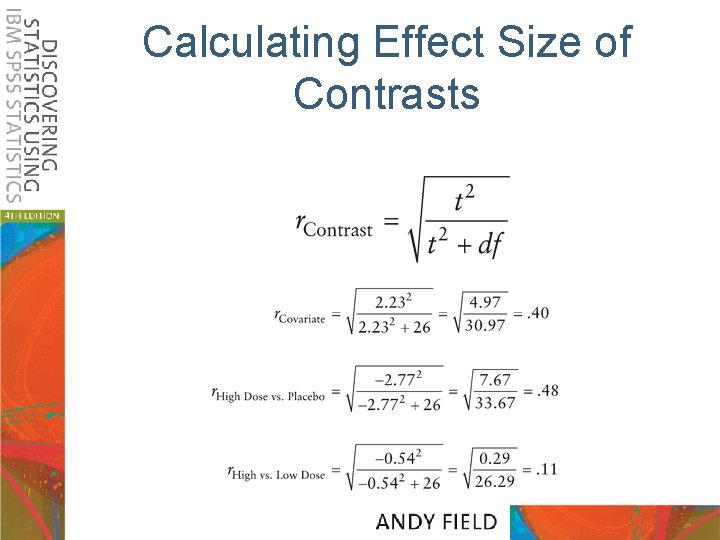
Calculating Effect Size of Contrasts

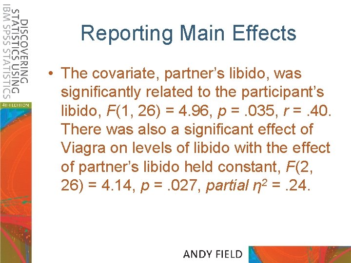
Reporting Main Effects • The covariate, partner’s libido, was significantly related to the participant’s libido, F(1, 26) = 4. 96, p =. 035, r =. 40. There was also a significant effect of Viagra on levels of libido with the effect of partner’s libido held constant, F(2, 26) = 4. 14, p =. 027, partial η 2 =. 24.

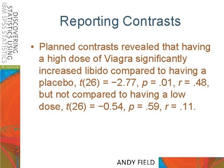
Reporting Contrasts • Planned contrasts revealed that having a high dose of Viagra significantly increased libido compared to having a placebo, t(26) = − 2. 77, p =. 01, r =. 48, but not compared to having a low dose, t(26) = − 0. 54, p =. 59, r =. 11.

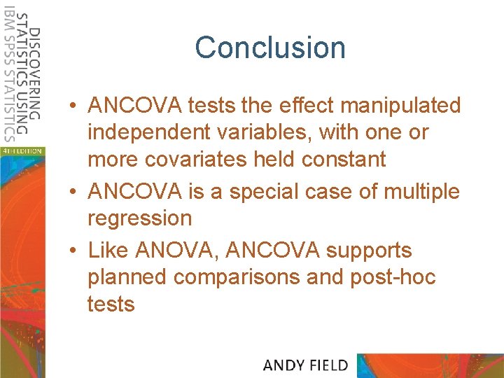
Conclusion • ANCOVA tests the effect manipulated independent variables, with one or more covariates held constant • ANCOVA is a special case of multiple regression • Like ANOVA, ANCOVA supports planned comparisons and post-hoc tests

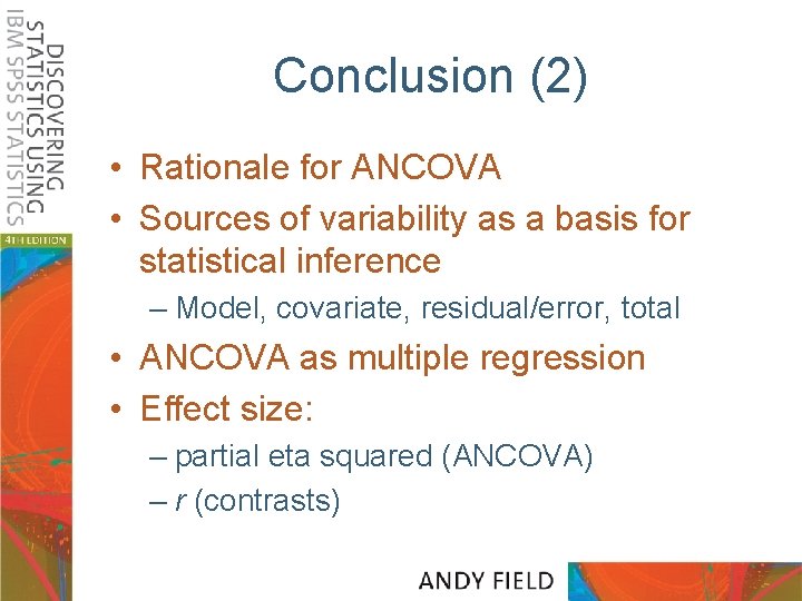
Conclusion (2) • Rationale for ANCOVA • Sources of variability as a basis for statistical inference – Model, covariate, residual/error, total • ANCOVA as multiple regression • Effect size: – partial eta squared (ANCOVA) – r (contrasts)