5 Joint Probability Distributions and Random Samples Copyright

Example: Joint pmf (discrete) The National Highway Traffic Safety Administration is interested in the effect of seat belt use on saving lives of children under 5. In this study, there were 7, 060 accidents where there was at least one fatality in the years between 1985 to 1989 (3015 children were involved). Let X denote whether the child survived or not and let Y denote the type of seat belt that the child wore (if any). The joint pmf of (X, Y) is given on the next slide.

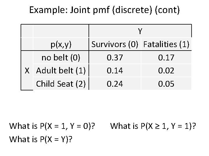
Example: Joint pmf (discrete) (cont) Y p(x, y) Survivors (0) Fatalities (1) no belt (0) 0. 37 0. 17 X Adult belt (1) 0. 14 0. 02 Child Seat (2) 0. 24 0. 05 What is P(X = 1, Y = 0)? What is P(X ≥ 1, Y = 1)? What is P(X = Y)?

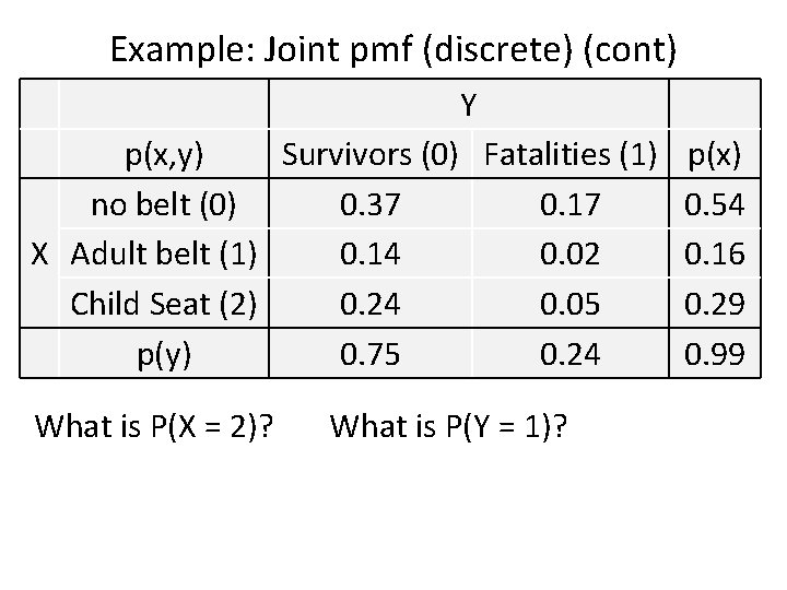
Example: Joint pmf (discrete) (cont) Y p(x, y) Survivors (0) Fatalities (1) p(x) no belt (0) 0. 37 0. 17 0. 54 X Adult belt (1) 0. 14 0. 02 0. 16 Child Seat (2) 0. 24 0. 05 0. 29 p(y) 0. 75 0. 24 0. 99 What is P(X = 2)? What is P(Y = 1)?

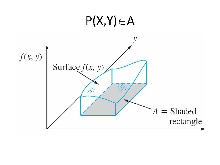
P(X, Y) A

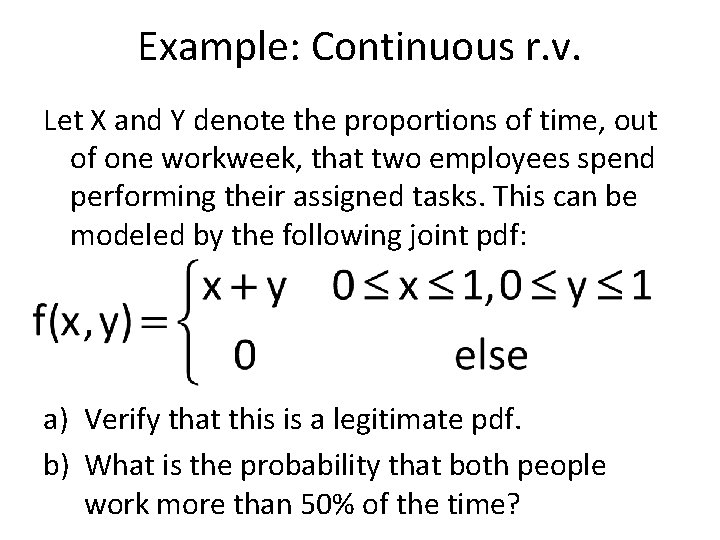
Example: Continuous r. v. Let X and Y denote the proportions of time, out of one workweek, that two employees spend performing their assigned tasks. This can be modeled by the following joint pdf: a) Verify that this is a legitimate pdf. b) What is the probability that both people work more than 50% of the time?

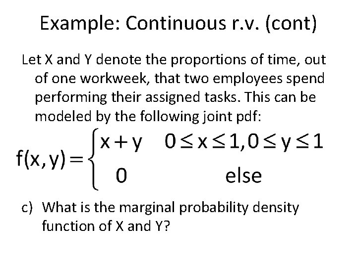
Example: Continuous r. v. (cont) Let X and Y denote the proportions of time, out of one workweek, that two employees spend performing their assigned tasks. This can be modeled by the following joint pdf: c) What is the marginal probability density function of X and Y?

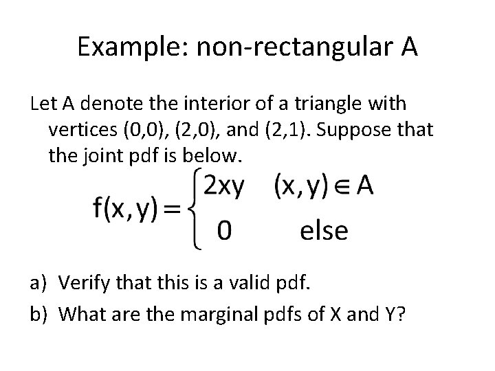
Example: non-rectangular A Let A denote the interior of a triangle with vertices (0, 0), (2, 0), and (2, 1). Suppose that the joint pdf is below. a) Verify that this is a valid pdf. b) What are the marginal pdfs of X and Y?

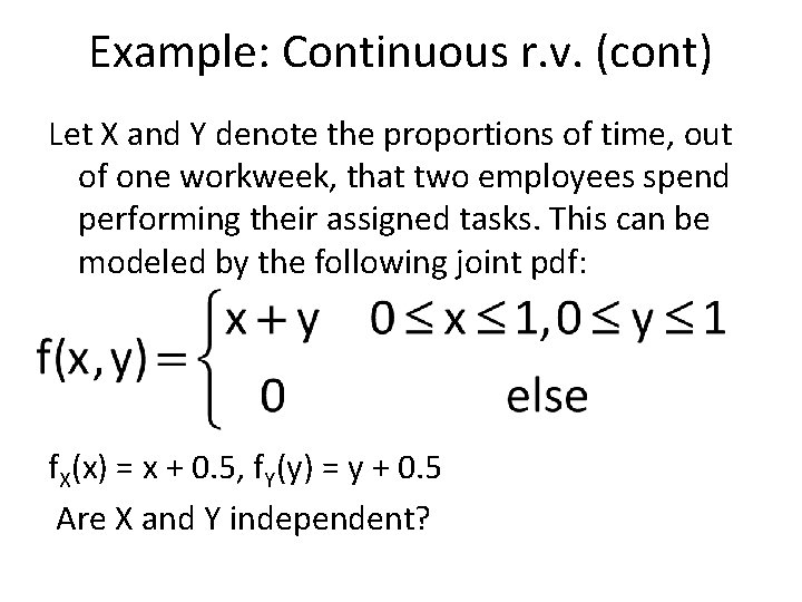
Example: Continuous r. v. (cont) Let X and Y denote the proportions of time, out of one workweek, that two employees spend performing their assigned tasks. This can be modeled by the following joint pdf: f. X(x) = x + 0. 5, f. Y(y) = y + 0. 5 Are X and Y independent?

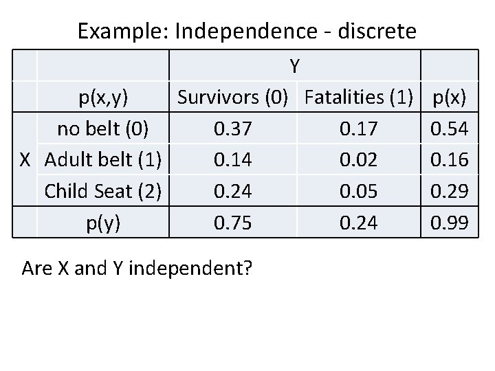
Example: Independence - discrete Y p(x, y) Survivors (0) Fatalities (1) p(x) no belt (0) 0. 37 0. 17 0. 54 X Adult belt (1) 0. 14 0. 02 0. 16 Child Seat (2) 0. 24 0. 05 0. 29 p(y) 0. 75 0. 24 0. 99 Are X and Y independent?

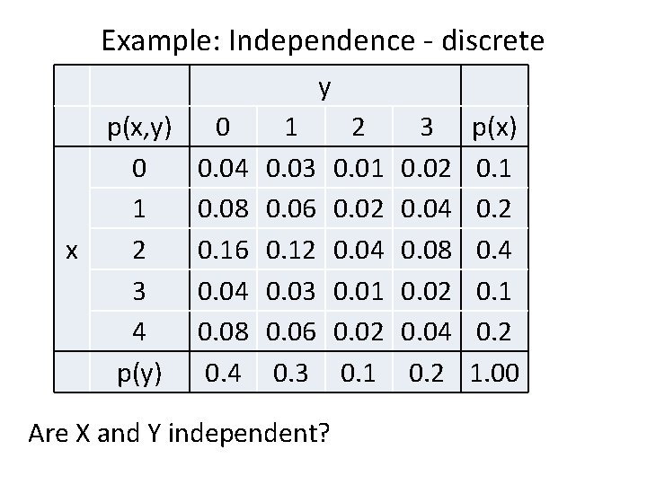
Example: Independence - discrete y x p(x, y) 0 1 2 3 4 p(y) 0 0. 04 0. 08 0. 16 0. 04 0. 08 0. 4 1 0. 03 0. 06 0. 12 0. 03 0. 06 0. 3 Are X and Y independent? 2 0. 01 0. 02 0. 04 0. 01 0. 02 0. 1 3 0. 02 0. 04 0. 08 0. 02 0. 04 0. 2 p(x) 0. 1 0. 2 0. 4 0. 1 0. 2 1. 00

Example: Independence X follows an exponential distribution with = 2; Y follows an exponential distribution with = 3. Assume that X and Y are independent. What is f(x, y)?

Multinomial Distribution •

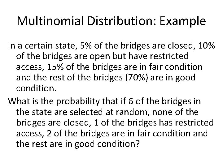
Multinomial Distribution: Example In a certain state, 5% of the bridges are closed, 10% of the bridges are open but have restricted access, 15% of the bridges are in fair condition and the rest of the bridges (70%) are in good condition. What is the probability that if 6 of the bridges in the state are selected at random, none of the bridges are closed, 1 of the bridges has restricted access, 2 of the bridges are in fair condition and the rest are in good condition?

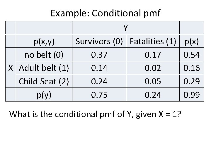
Example: Conditional pmf Y p(x, y) Survivors (0) Fatalities (1) p(x) no belt (0) 0. 37 0. 17 0. 54 X Adult belt (1) 0. 14 0. 02 0. 16 Child Seat (2) 0. 24 0. 05 0. 29 p(y) 0. 75 0. 24 0. 99 What is the conditional pmf of Y, given X = 1?

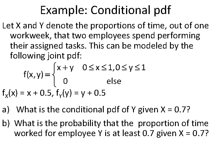
Example: Conditional pdf Let X and Y denote the proportions of time, out of one workweek, that two employees spend performing their assigned tasks. This can be modeled by the following joint pdf: f. X(x) = x + 0. 5, f. Y(y) = y + 0. 5 a) What is the conditional pdf of Y given X = 0. 7? b) What is the probability that the proportion of time worked for employee Y is at least 0. 7 given X = 0. 7?

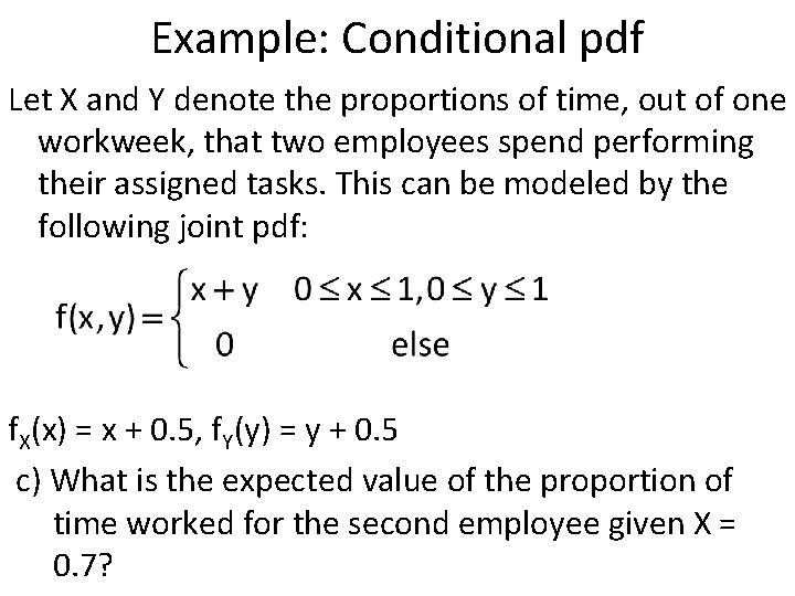
Example: Conditional pdf Let X and Y denote the proportions of time, out of one workweek, that two employees spend performing their assigned tasks. This can be modeled by the following joint pdf: f. X(x) = x + 0. 5, f. Y(y) = y + 0. 5 c) What is the expected value of the proportion of time worked for the second employee given X = 0. 7?

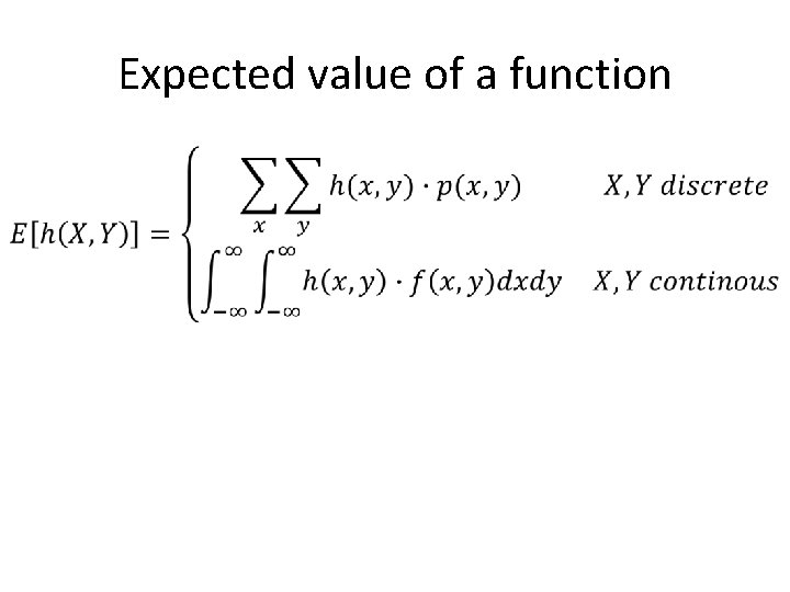
Expected value of a function •

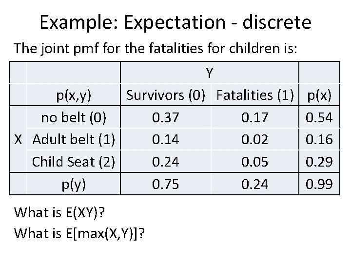
Example: Expectation - discrete The joint pmf for the fatalities for children is: Y p(x, y) Survivors (0) Fatalities (1) p(x) no belt (0) 0. 37 0. 17 0. 54 X Adult belt (1) 0. 14 0. 02 0. 16 Child Seat (2) 0. 24 0. 05 0. 29 p(y) 0. 75 0. 24 0. 99 What is E(XY)? What is E[max(X, Y)]?

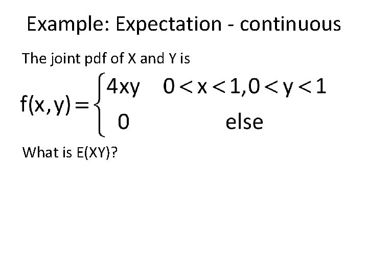
Example: Expectation - continuous The joint pdf of X and Y is What is E(XY)?

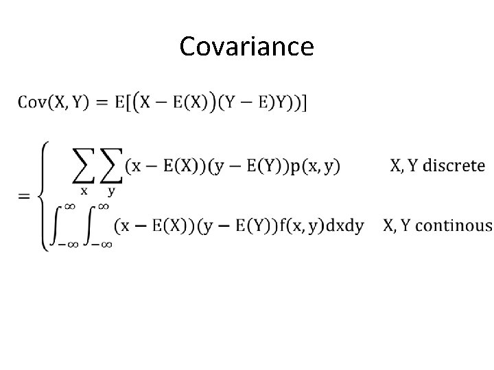
Covariance •

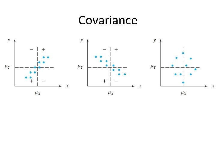
Covariance

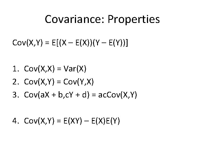
Covariance: Properties Cov(X, Y) = E[(X – E(X))(Y – E(Y))] 1. Cov(X, X) = Var(X) 2. Cov(X, Y) = Cov(Y, X) 3. Cov(a. X + b, c. Y + d) = ac. Cov(X, Y) 4. Cov(X, Y) = E(XY) – E(X)E(Y)

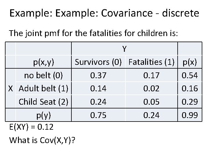
Example: Covariance - discrete The joint pmf for the fatalities for children is: Y p(x, y) Survivors (0) Fatalities (1) p(x) no belt (0) 0. 37 0. 17 0. 54 X Adult belt (1) 0. 14 0. 02 0. 16 Child Seat (2) 0. 24 0. 05 0. 29 p(y) 0. 75 0. 24 0. 99 E(XY) = 0. 12 What is Cov(X, Y)?

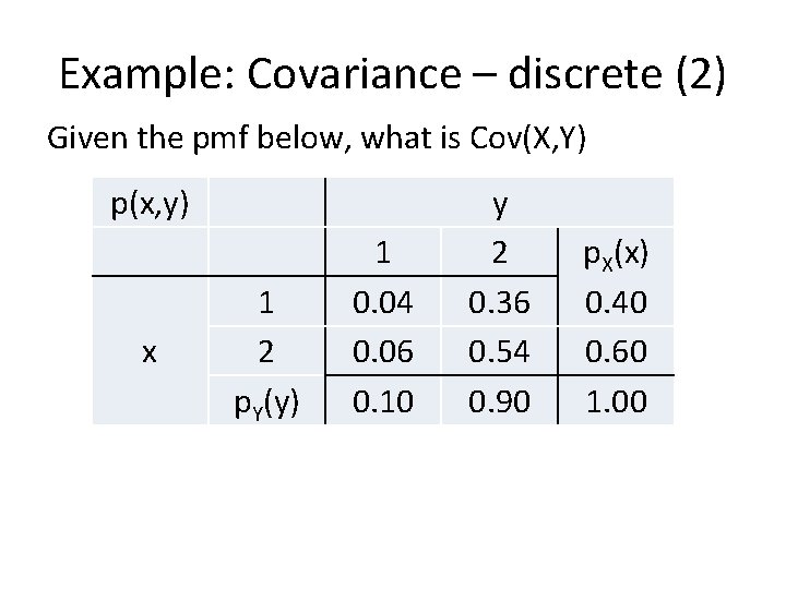
Example: Covariance – discrete (2) Given the pmf below, what is Cov(X, Y) p(x, y) x 1 2 p. Y(y) 1 0. 04 0. 06 0. 10 y 2 0. 36 0. 54 0. 90 p. X(x) 0. 40 0. 60 1. 00

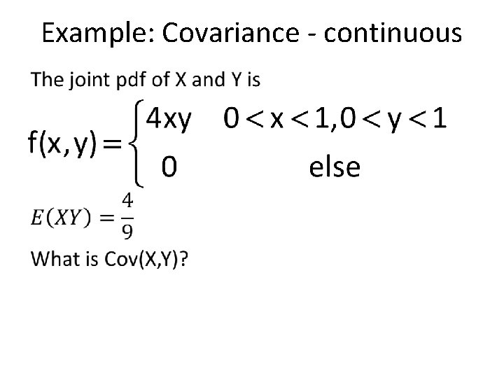
Example: Covariance - continuous •

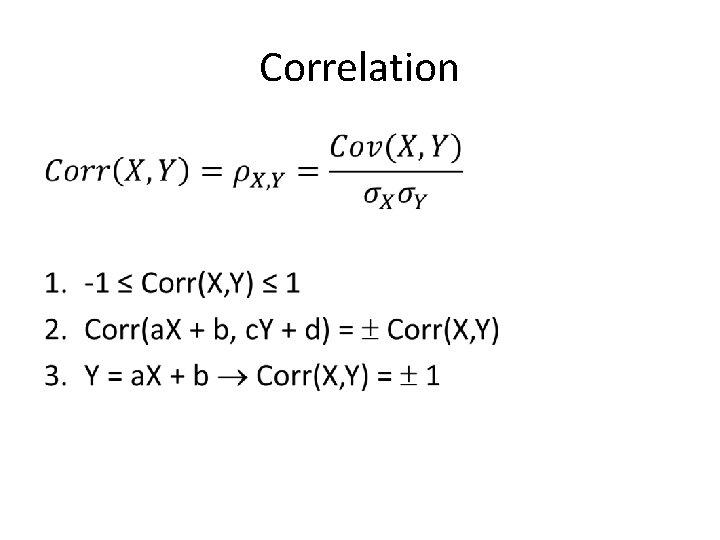
Correlation •

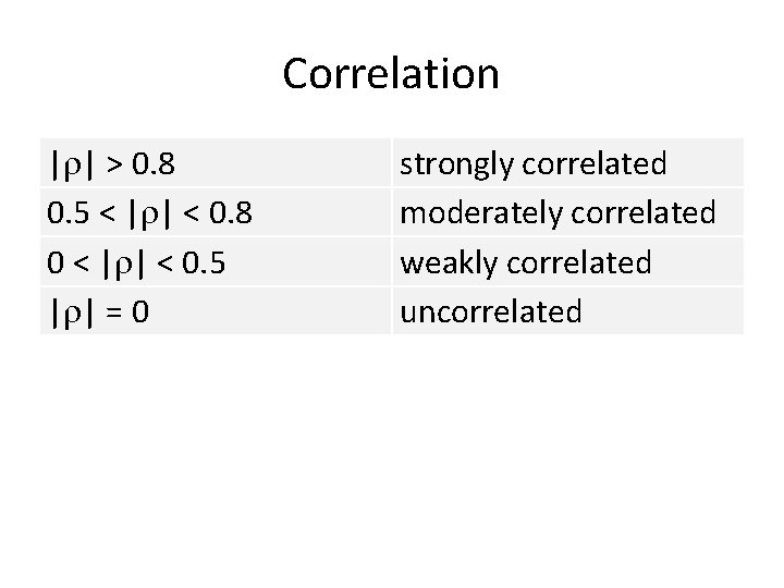
Correlation | | > 0. 8 0. 5 < | | < 0. 8 0 < | | < 0. 5 | | = 0 strongly correlated moderately correlated weakly correlated uncorrelated

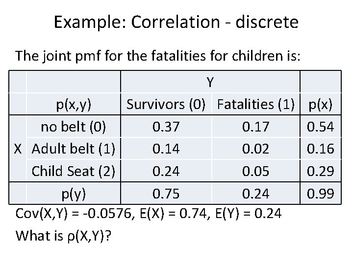
Example: Correlation - discrete The joint pmf for the fatalities for children is: Y p(x, y) Survivors (0) Fatalities (1) no belt (0) 0. 37 0. 17 X Adult belt (1) 0. 14 0. 02 Child Seat (2) 0. 24 0. 05 p(y) 0. 75 0. 24 Cov(X, Y) = -0. 0576, E(X) = 0. 74, E(Y) = 0. 24 What is ρ(X, Y)? p(x) 0. 54 0. 16 0. 29 0. 99

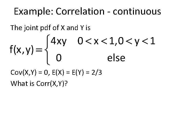
Example: Correlation - continuous The joint pdf of X and Y is Cov(X, Y) = 0, E(X) = E(Y) = 2/3 What is Corr(X, Y)?

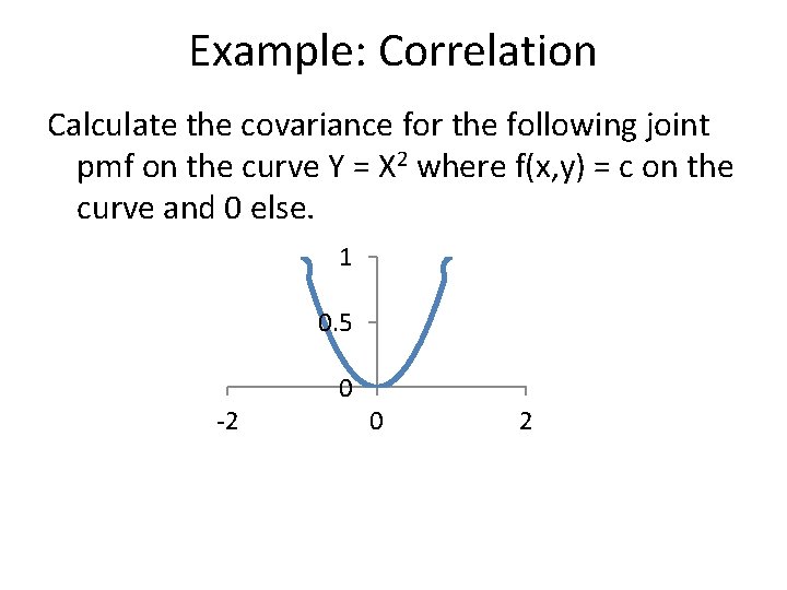
Example: Correlation Calculate the covariance for the following joint pmf on the curve Y = X 2 where f(x, y) = c on the curve and 0 else. 1 0. 5 -2 0 0 2

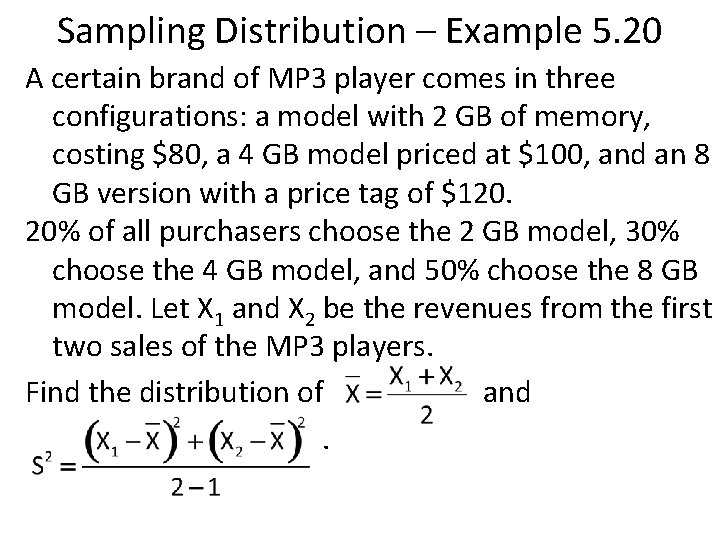
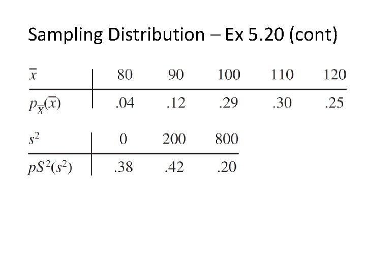
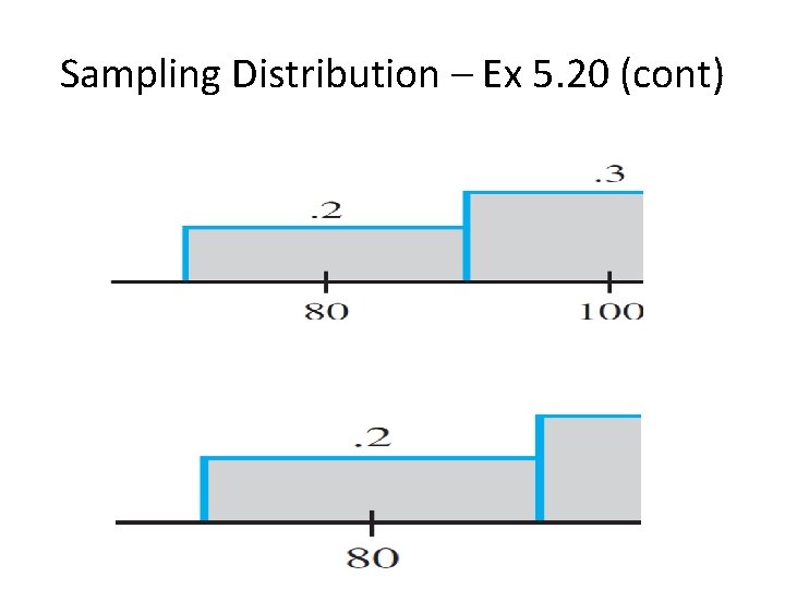
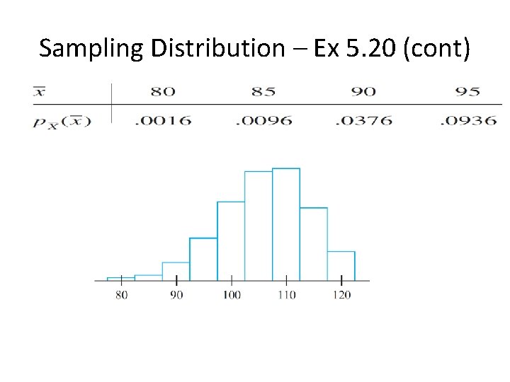
Sampling Distribution – Example 5. 20 A certain brand of MP 3 player comes in three configurations: a model with 2 GB of memory, costing $80, a 4 GB model priced at $100, and an 8 GB version with a price tag of $120. 20% of all purchasers choose the 2 GB model, 30% choose the 4 GB model, and 50% choose the 8 GB model. Let X 1 and X 2 be the revenues from the first two sales of the MP 3 players. Find the distribution of and .

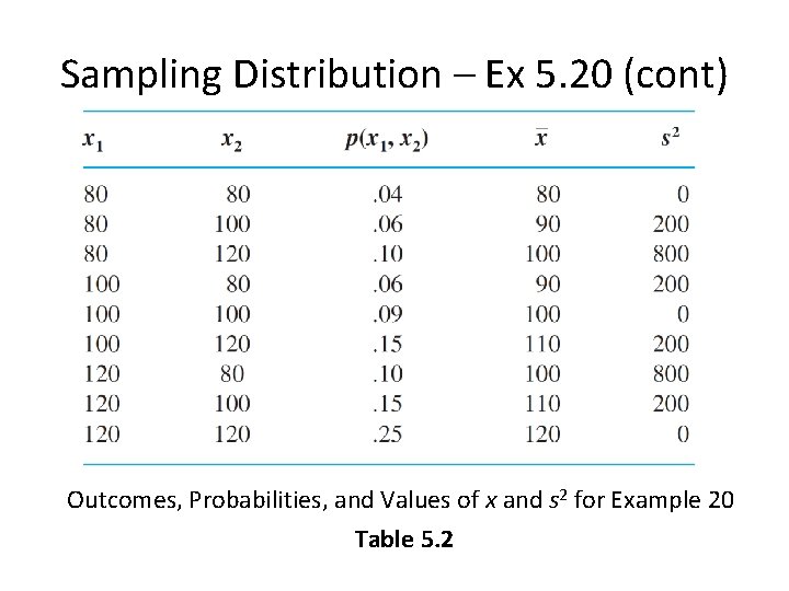
Sampling Distribution – Ex 5. 20 (cont) Outcomes, Probabilities, and Values of x and s 2 for Example 20 Table 5. 2

Sampling Distribution – Ex 5. 20 (cont)

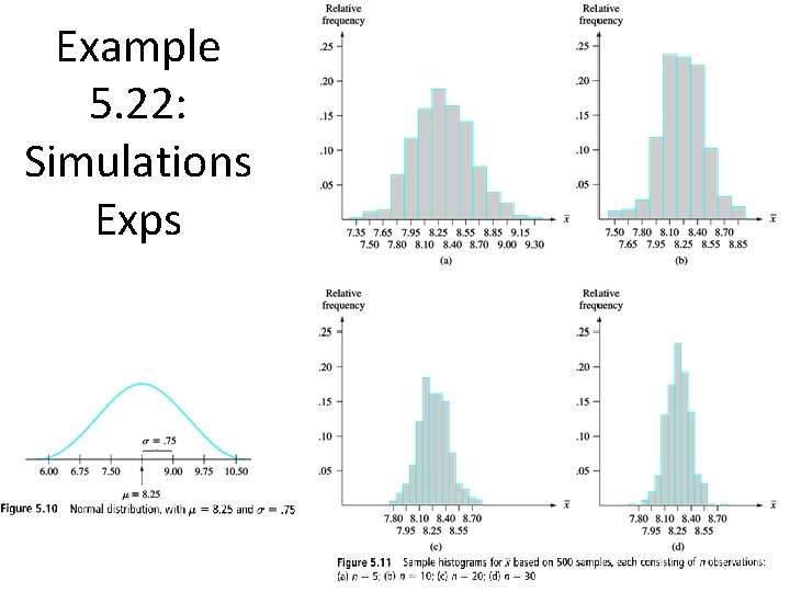
Example 5. 22: Simulations Exps

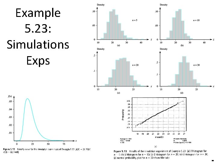
Example 5. 23: Simulations Exps

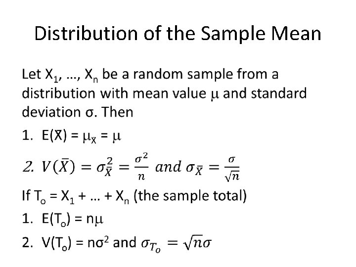
Distribution of the Sample Mean •

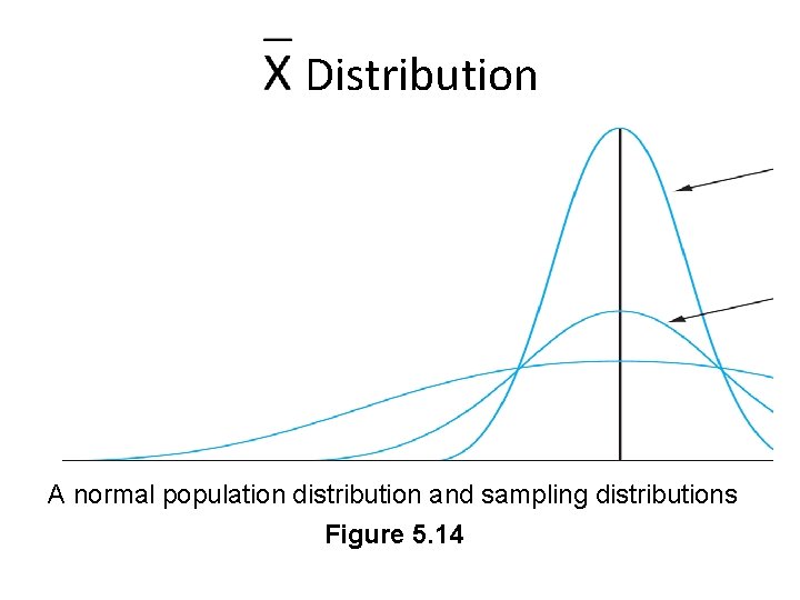
Distribution A normal population distribution and sampling distributions Figure 5. 14

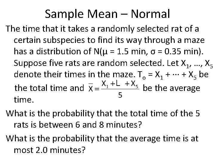
Sample Mean – Normal The time that it takes a randomly selected rat of a certain subspecies to find its way through a maze has a distribution of N(μ = 1. 5 min, σ = 0. 35 min). Suppose five rats are random selected. Let X 1, …, X 5 denote their times in the maze. To = X 1 + ∙∙∙ + X 5 be the total time and be the average time. What is the probability that the total time of the 5 rats is between 6 and 8 minutes? What is the probability that the average time is at most 2. 0 minutes?

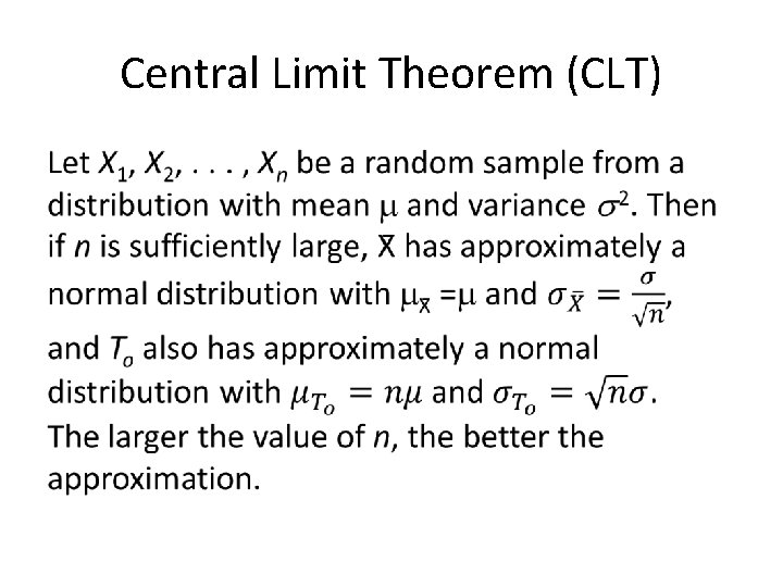
Central Limit Theorem (CLT) •

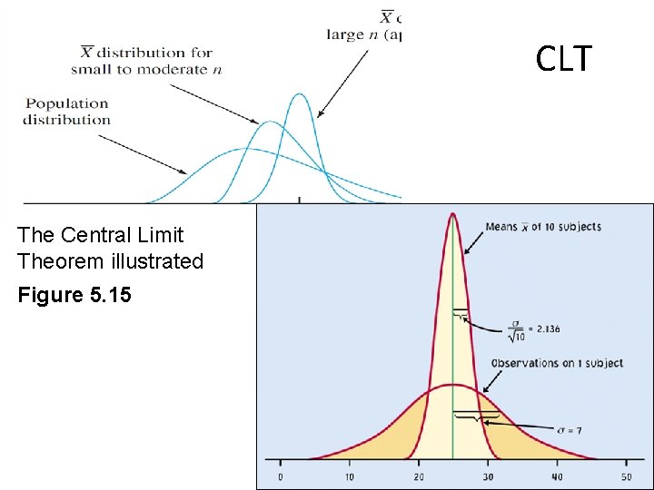
CLT The Central Limit Theorem illustrated Figure 5. 15

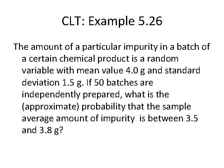
CLT: Example 5. 26 The amount of a particular impurity in a batch of a certain chemical product is a random variable with mean value 4. 0 g and standard deviation 1. 5 g. If 50 batches are independently prepared, what is the (approximate) probability that the sample average amount of impurity is between 3. 5 and 3. 8 g?

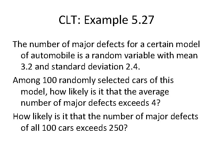
CLT: Example 5. 27 The number of major defects for a certain model of automobile is a random variable with mean 3. 2 and standard deviation 2. 4. Among 100 randomly selected cars of this model, how likely is it that the average number of major defects exceeds 4? How likely is it that the number of major defects of all 100 cars exceeds 250?

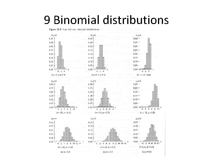
9 Binomial distributions

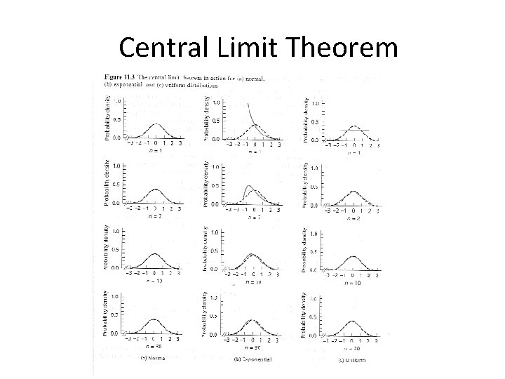
Central Limit Theorem

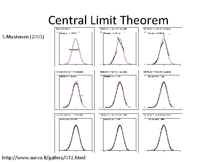
Central Limit Theorem S. Mustonen (2003) http: //www. survo. fi/gallery/072. html

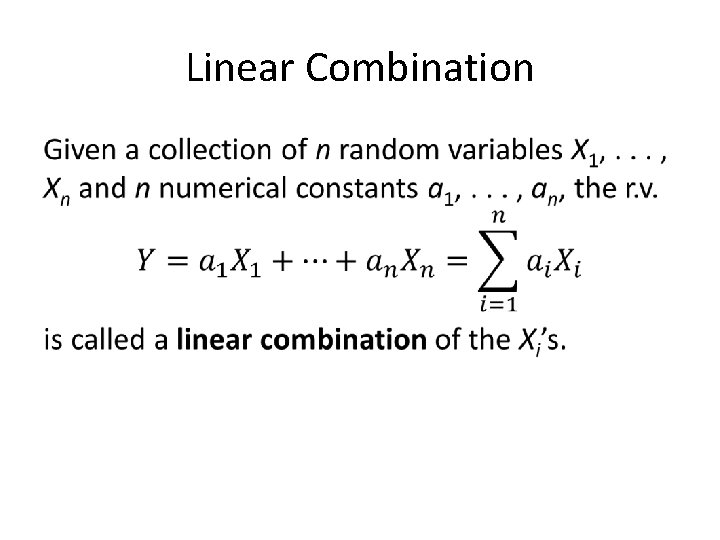
Linear Combination •

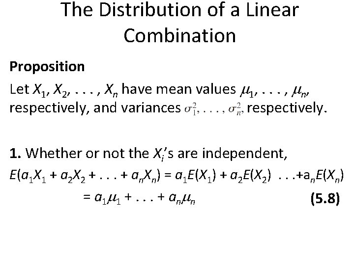
The Distribution of a Linear Combination Proposition Let X 1, X 2, . . . , Xn have mean values 1, . . . , n, respectively, and variances respectively. 1. Whether or not the Xi’s are independent, E(a 1 X 1 + a 2 X 2 +. . . + an. Xn) = a 1 E(X 1) + a 2 E(X 2) . . . +an. E(Xn) = a 1 1 +. . . + an n (5. 8)

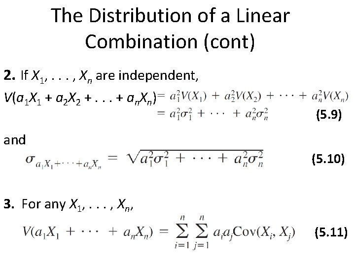
The Distribution of a Linear Combination (cont) 2. If X 1, . . . , Xn are independent, V(a 1 X 1 + a 2 X 2 +. . . + an. Xn) (5. 9) and (5. 10) 3. For any X 1, . . . , Xn, (5. 11)

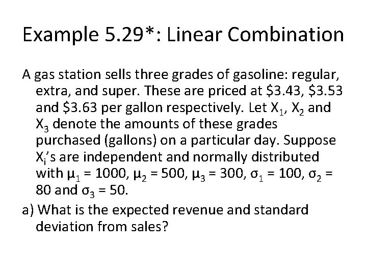
Example 5. 29*: Linear Combination A gas station sells three grades of gasoline: regular, extra, and super. These are priced at $3. 43, $3. 53 and $3. 63 per gallon respectively. Let X 1, X 2 and X 3 denote the amounts of these grades purchased (gallons) on a particular day. Suppose Xi’s are independent and normally distributed with μ 1 = 1000, μ 2 = 500, μ 3 = 300, σ1 = 100, σ2 = 80 and σ3 = 50. a) What is the expected revenue and standard deviation from sales?

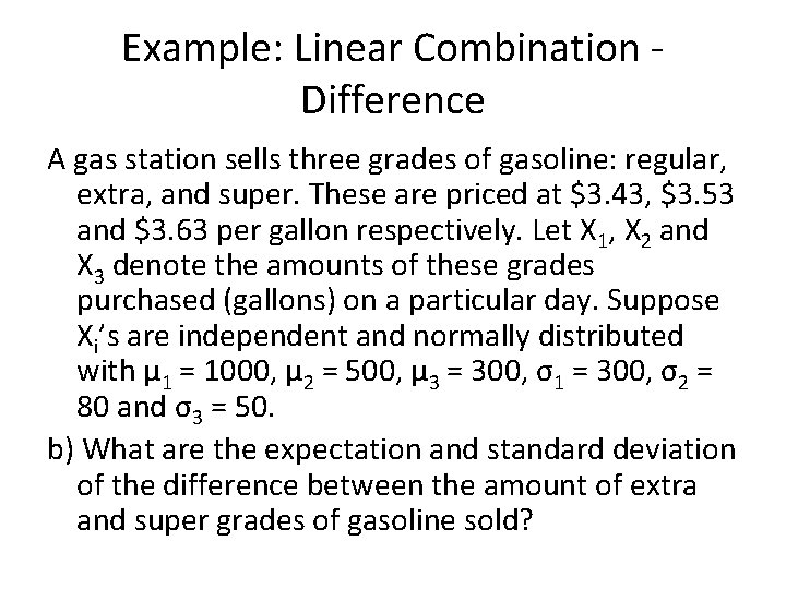
Example: Linear Combination - Difference A gas station sells three grades of gasoline: regular, extra, and super. These are priced at $3. 43, $3. 53 and $3. 63 per gallon respectively. Let X 1, X 2 and X 3 denote the amounts of these grades purchased (gallons) on a particular day. Suppose Xi’s are independent and normally distributed with μ 1 = 1000, μ 2 = 500, μ 3 = 300, σ1 = 300, σ2 = 80 and σ3 = 50. b) What are the expectation and standard deviation of the difference between the amount of extra and super grades of gasoline sold?

Example 5. 31*: Linear Combination - Normal A gas station sells three grades of gasoline: regular, extra, and super. These are priced at $3. 43, $3. 53 and $3. 63 per gallon respectively. Let X 1, X 2 and X 3 denote the amounts of these grades purchased (gallons) on a particular day. Suppose Xi’s are independent and normally distributed with μ 1 = 1000, μ 2 = 500, μ 3 = 300, σ1 = 100, σ2 = 80 and σ3 = 50. E(Y) = $6284. 00, Y = $479. 94 c) Find the probability that the total revenue exceeds $6000.