Analysis of continuous dynamical systems using statistical model

Analysis of continuous dynamical systems using statistical model checking P S Thiagarajan School of Computing National University of Singapore Joint work with: Sucheendra Palaniappan, Benjamin Gyori, Liu Bing, David Hsu

Continuous dynamical systems • Many physical systems interact with a digital controller. – automotive, avionics, manufacturing …. . • The key state variables will be real-valued evolving continuously over time. – Pressure, temperature, speed, … • The dynamics will be described by differential equations.

Differential equations x(0) = 2 The behavior of interest is the solution function. x(t) = t 3 + 4 t + x(0) = t 3 + 4 t + 2 x(t) 2

Plants and controllers PLANT actuators Sensors Digital Controller Plant dynamics: Differential equations Controller dynamics: Models of programs, ASICs, FPGAs, …. 4

PLANT actuators Sensors Digital Controller Given WCET analysis results what can we guarantee about the plant dynamics? Given the plant dynamics requirements (achieve stability within bounded time; stay only a bounded amount of time in a bad region) what should be the worst case performance? 5

E+S Initial concentrations : [E 0] = 9 nmol/l [S 0] = 13. 5 nmol/l [ES 0] = 0 nmol/l [P 0] = 0 nmol/l k 1 k 2 ES Rate constants : k 1 = 0. 1 l/(nmol*min) k 2 = 0. 1 min-1 k 3= 0. 3 min-1 k 3 E+P

Time (minutes) Concentration(n. M)

Where do we want to go with this?

Outline PART I – The behavior of a system of ODEs (ordinary differential equations). – A compact state space – IN, a set of initial states. – Behavior = TRJIN, the set of trajectories starting from IN.

Outline PART II – The specification logic. – BLTL (Bounded linear time temporal logic). – Interpreted at discrete time points: • 0, 1, 2, ……. , T – Finite discrete time horizon – Semantics:

Outline PART III – The (intractable) model checking problem: • TRJ = TRJIN ? • The probabilistic model checking problem: Pr(TRJ ) p ? – How to define Pr(TRJ How to define ) ? – C 1 continuity + theory of ODEs + measure theory

Outline PART IV – A statistical model checking (SMC) procedure to approximately solve “Pr(TRJ ) p ? ” PART V – A systems biology application

PART I: Behaviors S

PART I: Behaviors Reasonable constraint for physical and biological processes.

PART I: Behaviors Control systems must cope with a range of inputs The initial value of protein concentrations is usually a range of values.

PART I: Behaviors

PART I: TRJ – The set of trajectories. (t) IN 0 t The solution functions are trajectories. We want reason about all the trajectories.

PART II: Syntax of BLTL • BLTL – Bounded linear time temporal logic. • Syntax – ap = (i, l, u) is an atomic proposition. – At the current time point the value of the variable xi falls in the interval (l, u).

PART II: Syntax of BLTL

PART II: Semantics • We will interpret the formulas only at discrete time points: – 0, 1, 2, …. , T • Finite time horizon • For each there exists K (depends only on ) such that a prefix of length K of a model will determine if it is a model of . • Assume T is sufficiently large.

PART II: Semantics (t) 0 1 2 T The plant state will be sensed at only discrete time points. Experimental data will be available only at a finite number of time points.

PART II: Semantics

PART III: The model checking problem

E+S Initial concentrations : [E 0] = 9 nmol/l [S 0] = 13. 5 nmol/l [ES 0] = 0 nmol/l [P 0] = 0 nmol/l k 1 k 2 ES k 3 Rate constants : k 1 = 0. 1 l/(nmol*min) k 2 = 0. 1 min-1 k 3= 0. 3 min-1 It is impossible to solve this ODEs system explicitly. E+P

PART III: The probabilistic model checking problem. • Pr(TRJ ) p p (0, 1) • What does this mean? • A randomly selected trajectory in TRJ will be a model of with probability p. – Assuming a uniform distribution over IN. • NOTE: We are not trying to compute Pr(TRJ ).

PART III: The probabilistic model checking problem

PART III: The probabilistic model checking problem

PART III: The measurability of IN

PART III: Measurable functions Y

The flow functions

A simple observation

IN is measurable.

IN is measurable.

IN is measurable.

IN is measurable.

Part III: The result

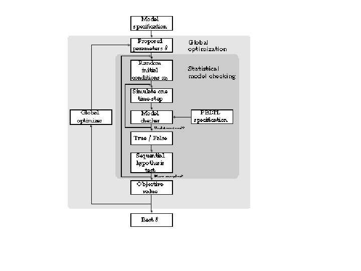
PART IV: The SMC procedure

Statistical model checking… •

Statistical model checking… •

Statistical model checking…

Sequential Probability Ratio Test (SPRT) [Wald, 1947] •

Sequential Probability Ratio Test (SPRT) [Wald, 1947]

PART IV: The SMC procedure

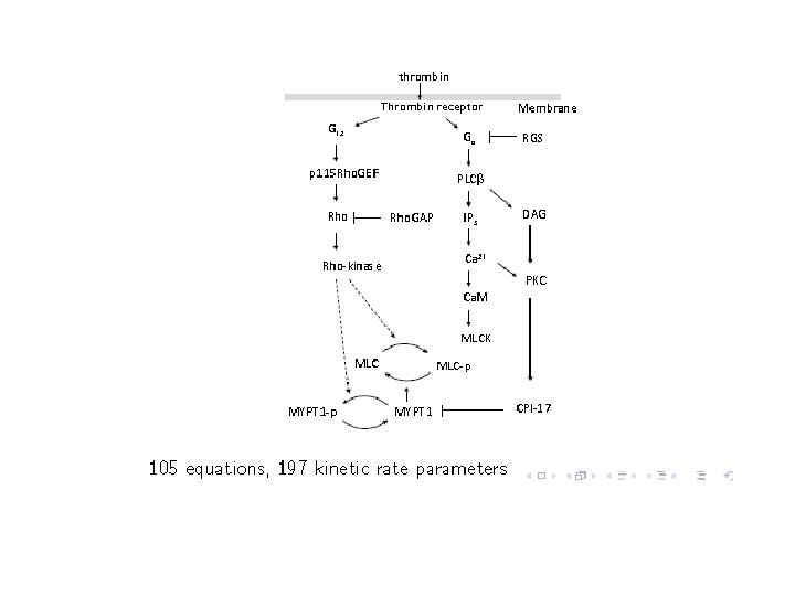
PART V: A systems biology application • Parameter estimation: – In an ODE model of a biochemical network many of the rate constants and initial concentrations (parameters) will be unknown. – One must estimate them using experimental data and some non-linear optimization technique.

E+S 0. 1 ES k 3 E+P

Parameter Estimation • Find values of parameter so that model prediction generated by simulations using these values can match experimental data krb. NGF = 0. 33, Km. Akt = 0. 16, kp. Raf 1 = 0. 42 … … target krb. NGF = 0. 49, Km. Akt = 0. 08, kp. Raf 1 = 0. 97 … … krb. NGF = 0. 88, Km. Akt = 0. 21, kp. Raf 1 = 0. 05 … … 11/27/2020 46

PART V: Parameter estimation • Randomly generate an initial set of parameter values • (A) Simulate and compare to experimental data. • (B) Update parameter values and repeat • How to update? – Most standard methods differ in the update phase, i. e. how to traverse the solution space 11/27/2020 47

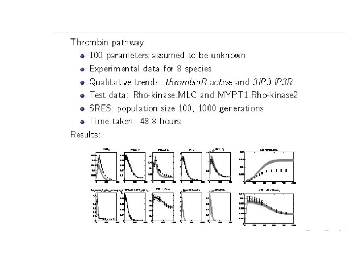
PART V: Parameter estimation • For step (A) we use our SMC procedure. – cell-to-cell variability – Experimental data is usually about a cell population. • Code up quantitative experimental data and qualitative trends as a formula . • Choose p, , , • Run SMC to determine if Pr p + ( ) • Update using an evolutionary strategy based algorithm called SRES.

PART V: Other applications • We have carried out similar studies on a number of other pathways. • We have also applied our SMC procedure to perform global sensitivity analysis. • Details can be found in: [Palaniappn et. al: CMSB’ 13]

Extension: Hybrid systems

Summary • Analyzing the dynamics of an ODEs system is an important task. – In control applications – In systems biology • The SMC procedure is approximate but scalable; based on simulations. • A significant opportunity formal verification technologies.

Summary • We are not advocating this methodology as an alternative to ``exact’’ verification. • But it could be used as an initial probe into the system dynamics. • Further, in many situations approximate verification may suffice or may be the only option.