Analisis de correspondencia linealizado Detrended Correspondence Analysis DCA

Analisis de correspondencia linealizado Detrended Correspondence Analysis (DCA)

Analisis de correspondencia • Promedios reciprocos • Se realiza el analisis en una matriz de siitios X especie (muestra X variables) • Se calculan los valores de las variables (especies) como combinaciones de los sitios en los que puedan ocurrir (distancias chi cuadrado) • Se calculan los valores de las muestras (sitios) usando combinaciones lineales de las especies • Se realiza una descomposición de la matriz similar a PCA (descomposición singular), maximiza correspondencia entre filas y columnas

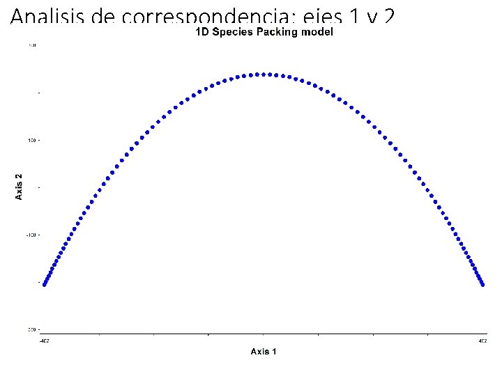
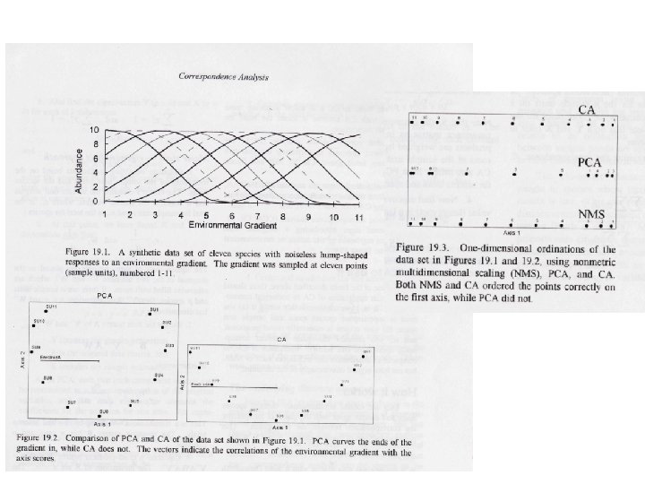
Problemas con CA y PCA en distribuciones sesgadas • “Efecto de arco”: una sequencia de muestras-sitios aparece deformarse en una curva cuando la variación es solo a lo largo de un gradiente • El orden de las muestras es correcto en el eje 1 pero las distancias entre ellas se comprimen a medida que las muestras alcanzan los extremos del gradiente • Cuando las muestras se encuentran a lo largo de mas de un gradiente la deformación en el primer gradiente oscurece las relaciones de los sitios-muestras sobre el Segundo gradiente.

Analisis de correspondencia: ejes 1 v 2

Analisis de correspondencia linealizado Detrended Correspondence Analysis (DCA) • Hill & Gauch (1980) • Modificacion del CA con la intención de remover “el efecto de arco” y corregir la compresión de los extremos de los gradientes • El mayor exito es que fue distribuido con DECORANA (Hill 1979) uno de los primeros programas en computadora • DCA todavia es usado a pesar de ciertas limitaciones

DCA no es un metodo es un Analisis de correspondencia CA modificado 1. Linealización: se realiza para remover la relación entre los valores de los sitios-muestras y los ejes de ordenación 2. Reescalamiento: ajuste no-linear de escalamiento en el primer eje para tener una cantidad constante de recambio de las especies entre sitios

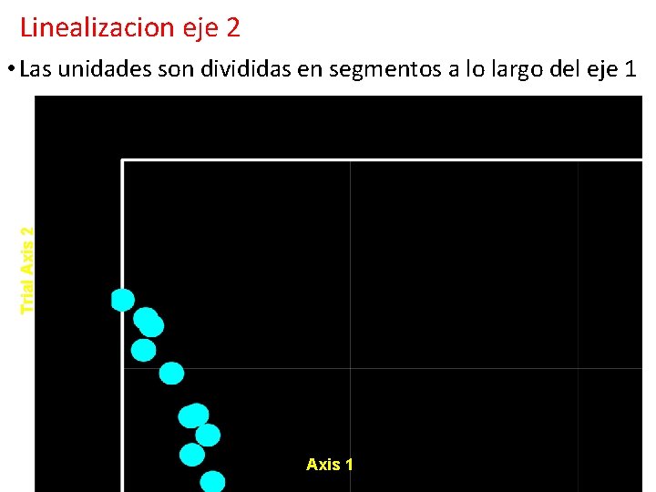
Linealizacion eje 2 Trial Axis 2 • Las unidades son divididas en segmentos a lo largo del eje 1 Axis 1

Linealizacion eje 2 Trial Axis 2 • El promedio del valor sobre el eje 2 es ajustado a 0 en cada segmento • La linealizacion es lelvada a cabo en cada iteración del proceso Axis 1

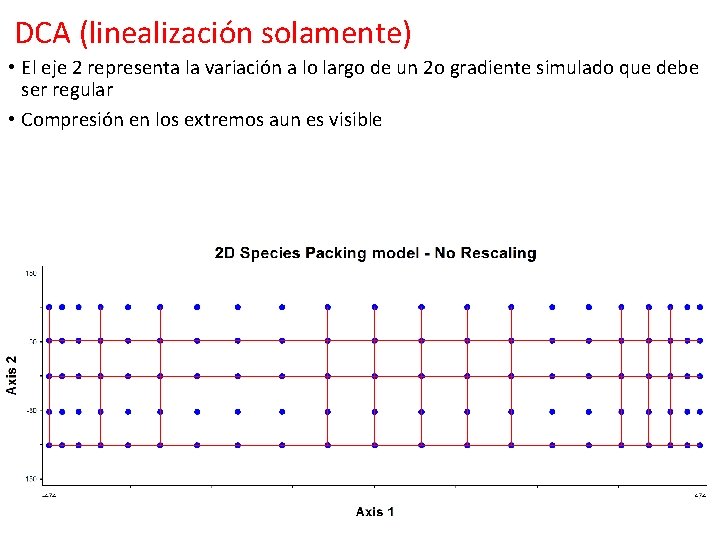
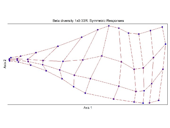
DCA (linealización solamente) • El eje 2 representa la variación a lo largo de un 2 o gradiente simulado que debe ser regular • Compresión en los extremos aun es visible

Reescalamiento • Transformación de los valores para que la tasa de cambio en la composición de especies sea constant a lo largo del eje 1 • Se logra expandiendo o contrayendo el escalamiento del primer eje de manera artificial • El reescalamiento se produce de tal manera que el ambiente representado se divide en un numero determinado de desviaciones standard (SD)

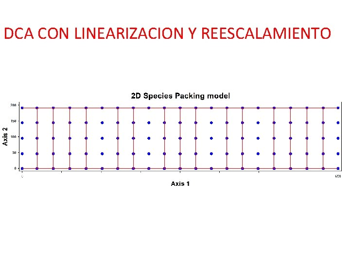
DCA CON LINEARIZACION Y REESCALAMIENTO

Autovalores en DCA (eigenvalues) • Los autovalores no representan la variabilidad ya que estos son calculados antes de los procesos de linearización y reescalamiento • No es compatible el procedimiento en los ejes 1 y 2 • Finalmente hay un reescalamiento para disminuir la influencia de especies raras

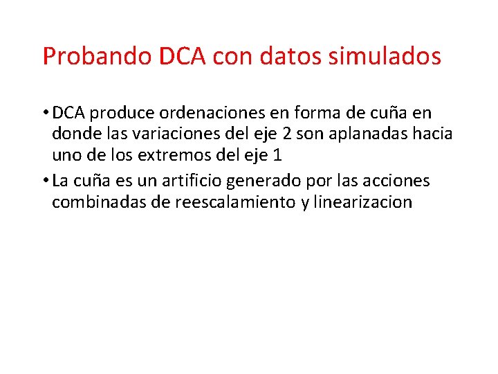
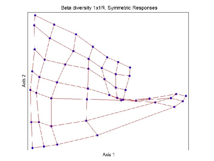
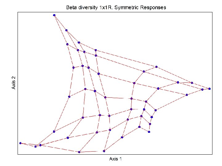
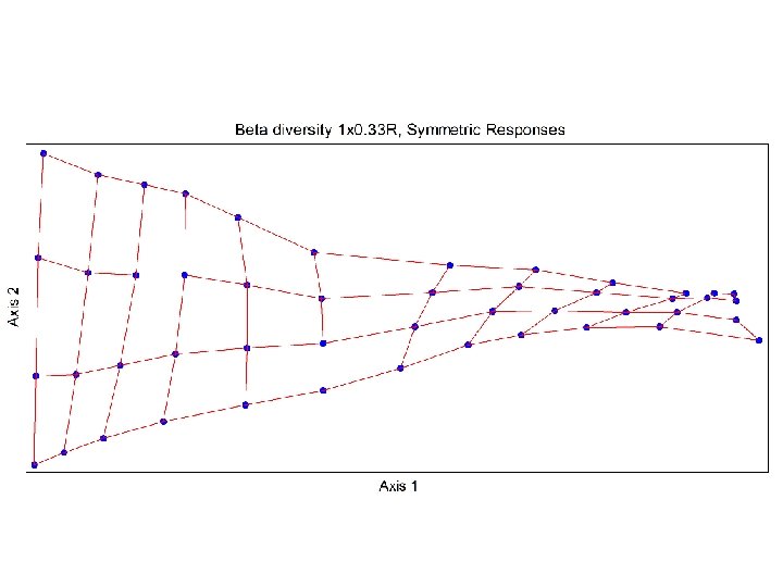
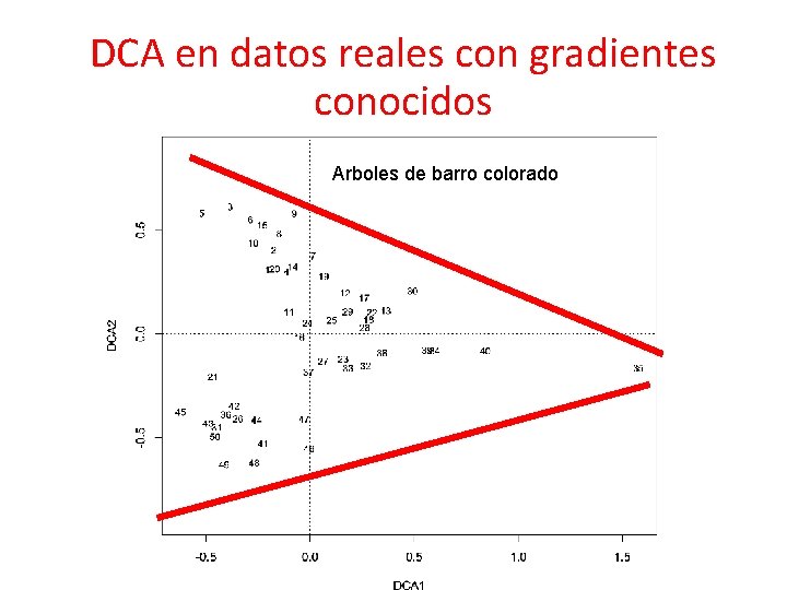
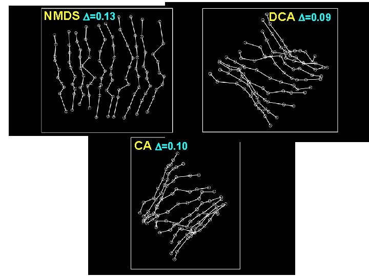
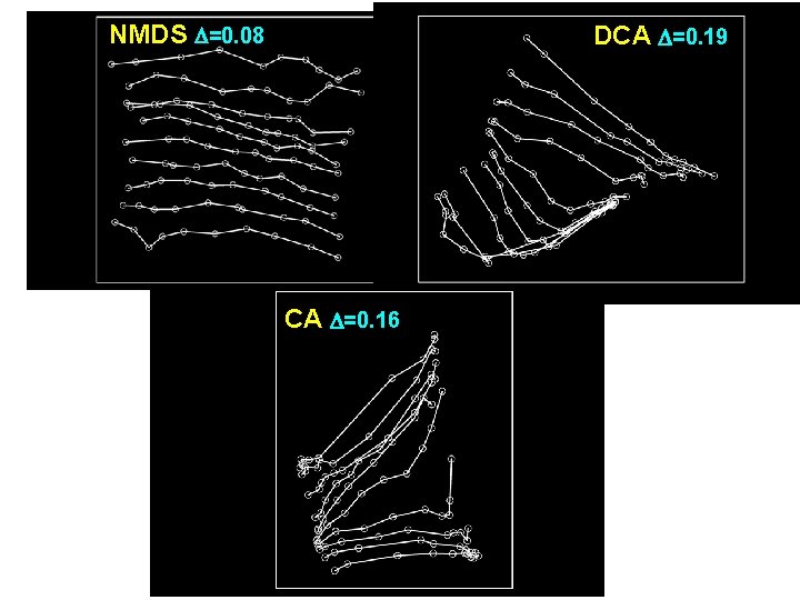
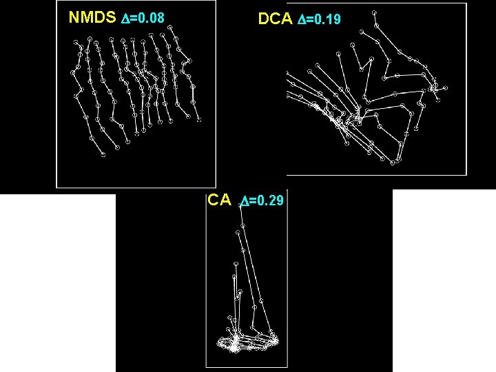
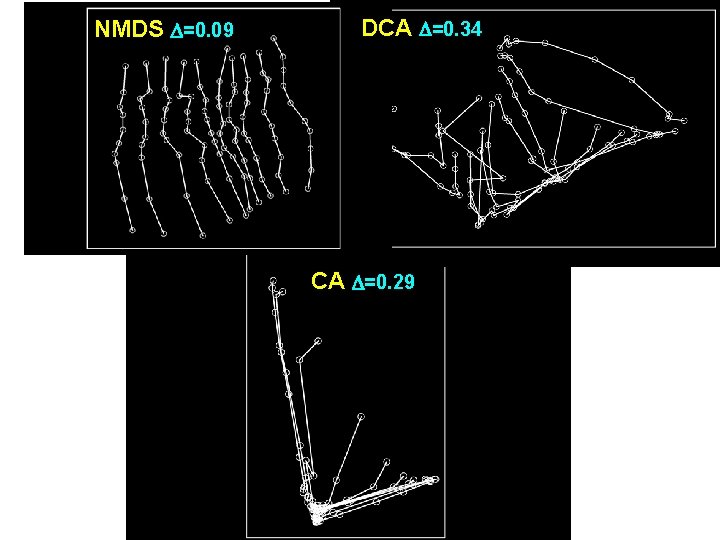
Probando DCA con datos simulados • DCA produce ordenaciones en forma de cuña en donde las variaciones del eje 2 son aplanadas hacia uno de los extremos del eje 1 • La cuña es un artificio generado por las acciones combinadas de reescalamiento y linearizacion

DCA en datos reales con gradientes conocidos Arboles de barro colorado

Nonmetric Multidimensional Scaling (NMDS) Escalamiento no metrico multidimensional

Escalamiento no metrico multidimensional • Developed by Shepard (1962) and Kruskal (1964) for psychological data • First applied in ecology by Anderson (1971) • Based on a fundamentally different approach than the eigenanalysis methods PCA, CA (and DCA) • Axes of NMDS are not rotated axes of a high-dimensional “species space”.

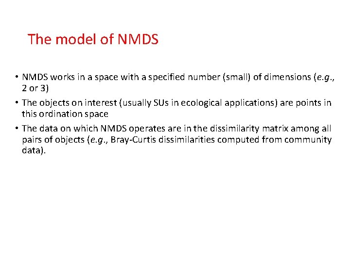
The model of NMDS • NMDS works in a space with a specified number (small) of dimensions (e. g. , 2 or 3) • The objects on interest (usually SUs in ecological applications) are points in this ordination space • The data on which NMDS operates are in the dissimilarity matrix among all pairs of objects (e. g. , Bray-Curtis dissimilarities computed from community data).

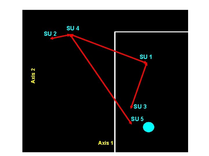
The model of NMDS • NMDS seeks an ordination in which the distances between all pairs of SUs are, as far as possible, in rank-order agreement with their dissimilarities in species composition.

SU 2 SU 4 Axis 2 SU 1 SU 3 SU 5 Axis 1

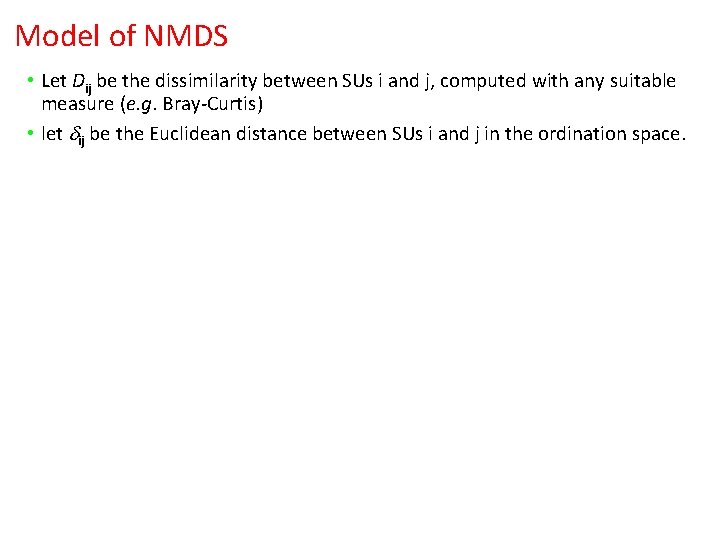
Model of NMDS • Let Dij be the dissimilarity between SUs i and j, computed with any suitable measure (e. g. Bray-Curtis) • let ij be the Euclidean distance between SUs i and j in the ordination space.

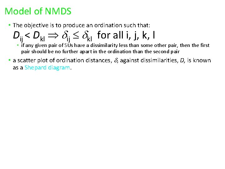
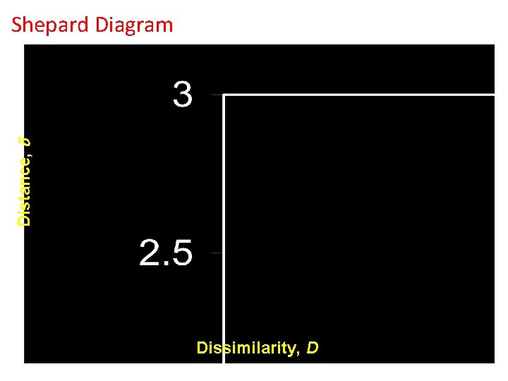
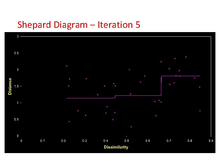
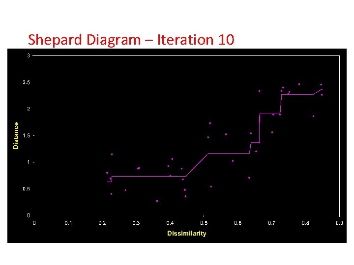
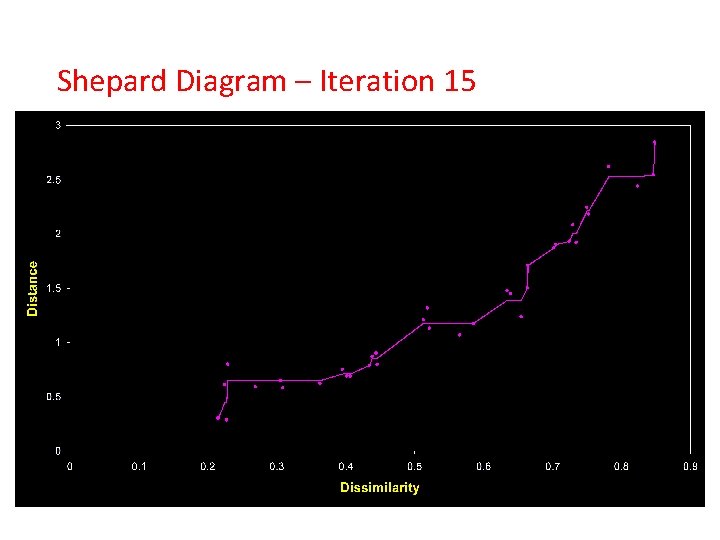
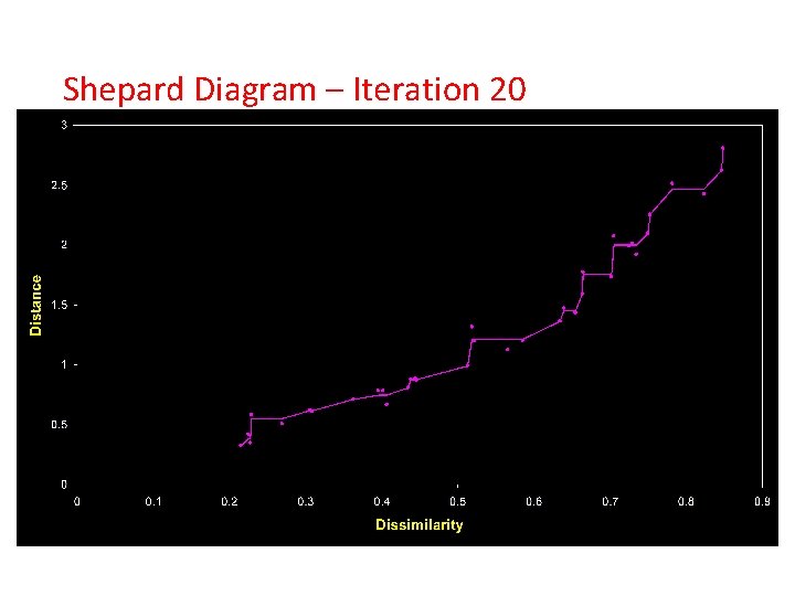
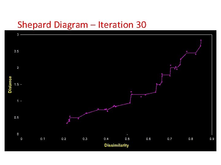
Model of NMDS • The objective is to produce an ordination such that: Dij < Dkl ij kl for all i, j, k, l • if any given pair of SUs have a dissimilarity less than some other pair, then the first pair should be no further apart in the ordination than the second pair • a scatter plot of ordination distances, , against dissimilarities, D, is known as a Shepard diagram.

Distance, Shepard Diagram Dissimilarity, D

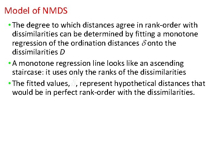
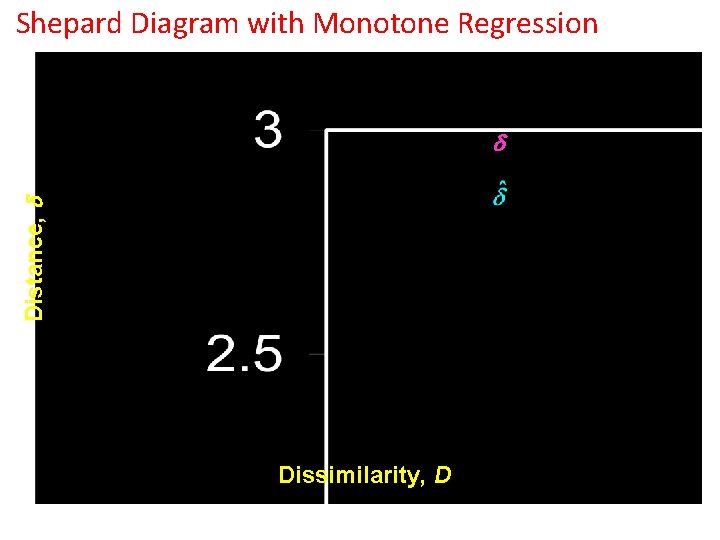
Model of NMDS • The degree to which distances agree in rank-order with dissimilarities can be determined by fitting a monotone regression of the ordination distances onto the dissimilarities D • A monotone regression line looks like an ascending staircase: it uses only the ranks of the dissimilarities • The fitted values, , represent hypothetical distances that would be in perfect rank-order with the dissimilarities.

Shepard Diagram with Monotone Regression Distance, Dissimilarity, D

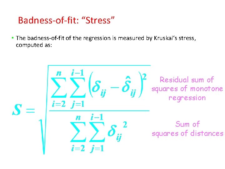
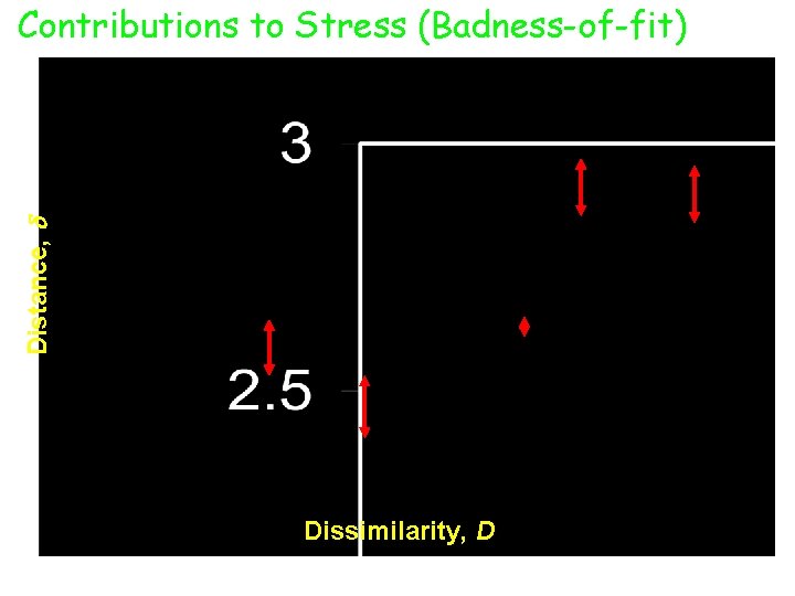
Badness-of-fit: “Stress” • The badness-of-fit of the regression is measured by Kruskal’s stress, computed as: Residual sum of squares of monotone regression Sum of squares of distances

Distance, Contributions to Stress (Badness-of-fit) Dissimilarity, D

Model of NMDS • Stress decreases as the rank-order agreement between distances and dissimilarities improves • The aim is therefore to find the ordination with the lowest possible stress • There is no algebraic solution to find the best ordination: it must be sought by an iterative search or trial-and-error optimization process.

Basic Algorithm for NMDS 1. Compute dissimilarities, D, among the n SUs using a suitable choice of data standardization and dissimilarity measure 2. Specify the number of ordination dimensions to be used 3. Generate an initial ordination of the SUs (starting configuration) with this number of axes • This can be totally random or an ordination of the SUs by some other method might be used.

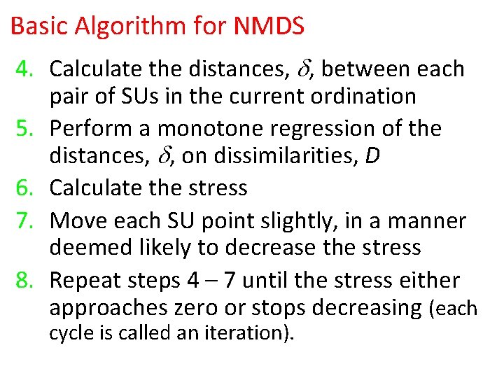
Basic Algorithm for NMDS 4. Calculate the distances, , between each 5. 6. 7. 8. pair of SUs in the current ordination Perform a monotone regression of the distances, , on dissimilarities, D Calculate the stress Move each SU point slightly, in a manner deemed likely to decrease the stress Repeat steps 4 – 7 until the stress either approaches zero or stops decreasing (each cycle is called an iteration).

Basic Algorithm for NMDS • Any suitable optimization method can be used at step 7 to decide how to move each point • Stress can be considered a function with many independent variables: the coordinates of each SU on each axis • The aim is to find the coordinates that will minimize this function • This is a difficult problem to solve, especially when n is large.

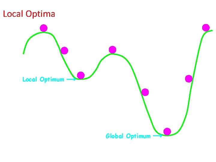
Local Optima • There is no guarantee that the ordination with the lowest possible stress (global optimum) will be found from any given initial ordination • The search may arrive at a local optimum, where no small change in any coordinates will make stress decrease, even though a solution with lower stress does exist.

Local Optima Local Optimum Global Optimum

Local Optima • run the entire ordination from several different starting configurations (typically at least 100) • if the algorithm converges to the same minimum stress solution from several different random starts, one can be confident the global optimum has been found.

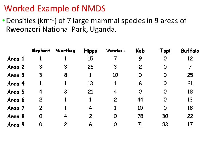
Worked Example of NMDS • Densities (km-1) of 7 large mammal species in 9 areas of Rweonzori National Park, Uganda. Elephant Warthog Hippo Waterbuck Kob Topi Buffalo Area 1 15 7 9 0 12 Area 2 3 3 28 3 2 0 7 Area 3 3 8 1 10 0 0 25 Area 4 1 1 13 1 6 0 21 Area 5 4 3 21 4 0 0 18 Area 6 2 1 1 2 44 0 13 Area 7 2 1 4 1 10 0 18 Area 8 0 4 2 0 78 30 22 Area 9 0 2 6 0 71 83 17

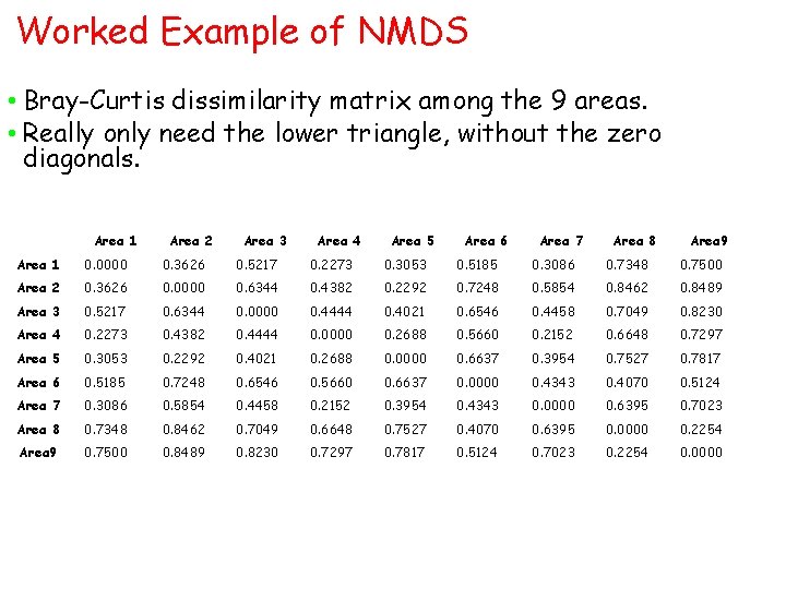
Worked Example of NMDS • Bray-Curtis dissimilarity matrix among the 9 areas. • Really only need the lower triangle, without the zero diagonals. Area 1 Area 2 Area 3 Area 4 Area 5 Area 6 Area 7 Area 8 Area 9 Area 1 0. 0000 0. 3626 0. 5217 0. 2273 0. 3053 0. 5185 0. 3086 0. 7348 0. 7500 Area 2 0. 3626 0. 0000 0. 6344 0. 4382 0. 2292 0. 7248 0. 5854 0. 8462 0. 8489 Area 3 0. 5217 0. 6344 0. 0000 0. 4444 0. 4021 0. 6546 0. 4458 0. 7049 0. 8230 Area 4 0. 2273 0. 4382 0. 4444 0. 0000 0. 2688 0. 5660 0. 2152 0. 6648 0. 7297 Area 5 0. 3053 0. 2292 0. 4021 0. 2688 0. 0000 0. 6637 0. 3954 0. 7527 0. 7817 Area 6 0. 5185 0. 7248 0. 6546 0. 5660 0. 6637 0. 0000 0. 4343 0. 4070 0. 5124 Area 7 0. 3086 0. 5854 0. 4458 0. 2152 0. 3954 0. 4343 0. 0000 0. 6395 0. 7023 Area 8 0. 7348 0. 8462 0. 7049 0. 6648 0. 7527 0. 4070 0. 6395 0. 0000 0. 2254 Area 9 0. 7500 0. 8489 0. 8230 0. 7297 0. 7817 0. 5124 0. 7023 0. 2254 0. 0000

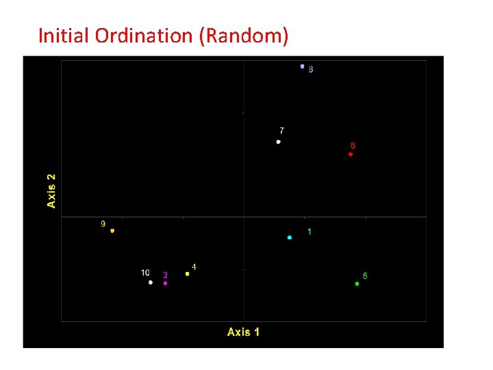
Initial Ordination (Random)

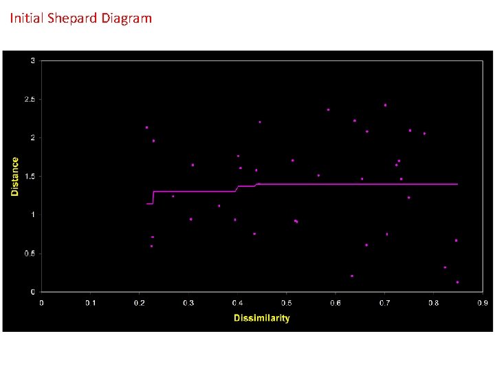
Initial Shepard Diagram

Stress • stress of initial (random) ordination is 0. 4183 • This is high, reflecting the poor rank-order agreement of distances with dissimilarities at this stage. • each SU point is now moved slightly

Axis 2 How the ordination evolved Axis 1

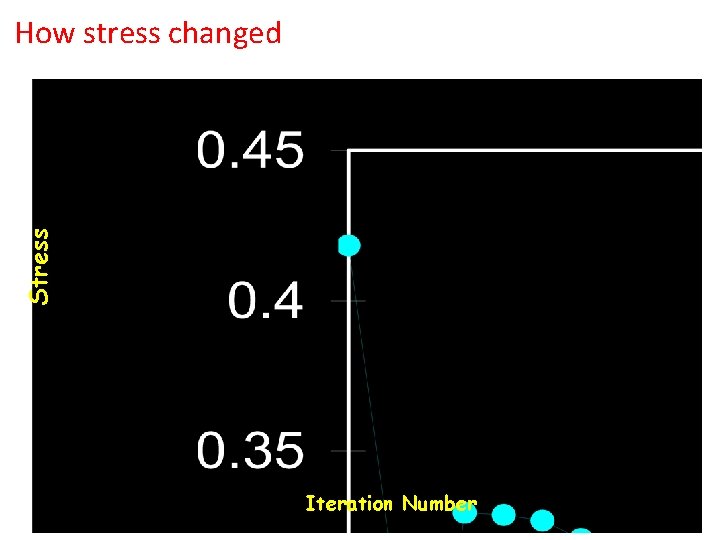
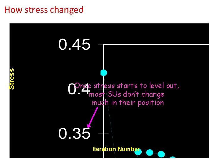
Stress How stress changed Iteration Number

Shepard Diagram – Iteration 5

Shepard Diagram – Iteration 10

Shepard Diagram – Iteration 15

Shepard Diagram – Iteration 20

Shepard Diagram – Iteration 30

Axis 2 How the ordination evolved Axis 1

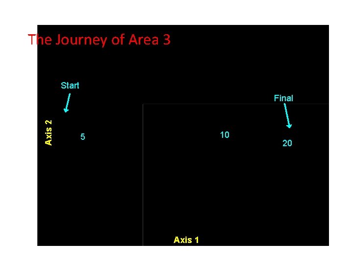
The Journey of Area 3 Start Axis 2 Final 10 5 Axis 1 20

Stress How stress changed Once stress starts to level out, most SUs don’t change much in their position Iteration Number

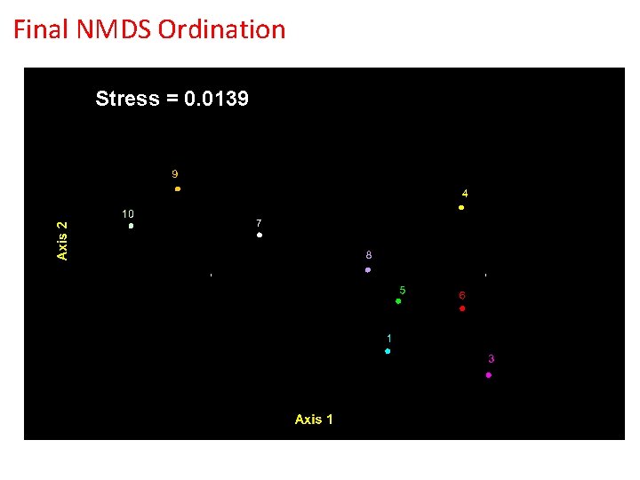
Final NMDS Ordination Stress = 0. 0139

Dimensionality • There is no way of knowing in advance how many dimensions you need for a given data set • To determine how many dimensions are needed, NMDS must be run in a range of dimensionalities • The vast majority of community data sets can be adequately summarized with 2 or 3 NMDS axes; rarely 4 or 5 may be needed.

Dimensionality • no simple relationship between axes in NMDS solutions for different numbers of dimensions • e. g. axes 1 and 2 of a 3 -D NMDS are not the same as axes 1 and 2 of the 2 -D solution • always possible to achieve a lower stress with an increase in dimensionality

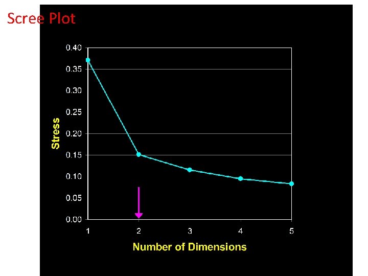
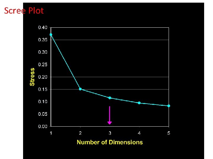
Scree Plots • A line plot of minimum stress (Y axis) against number of dimensions is called a scree plot • It can be used as a guide in deciding on the number of dimensions required • A sharp break in slope of the curve, beyond which further reductions in stress are small, suggests dimensionality.

Scree Plot

Scree Plot

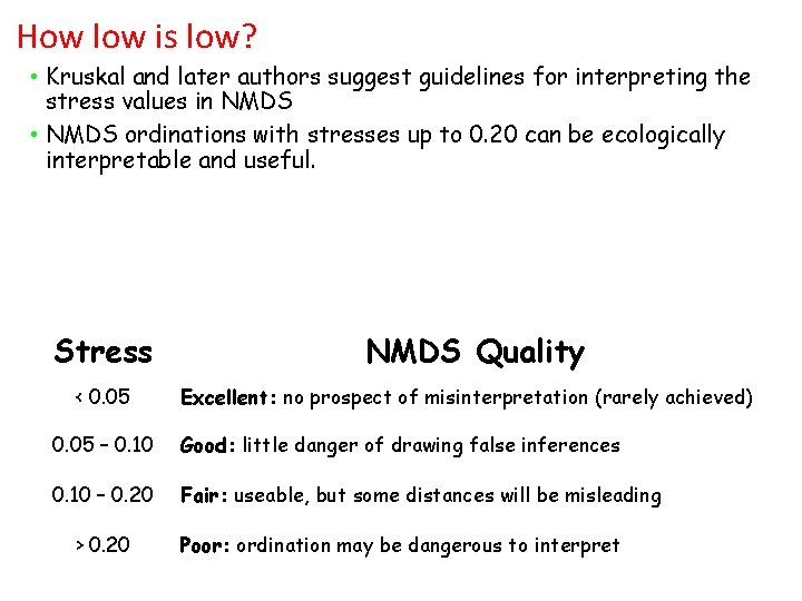
How low is low? • Kruskal and later authors suggest guidelines for interpreting the stress values in NMDS • NMDS ordinations with stresses up to 0. 20 can be ecologically interpretable and useful. Stress < 0. 05 NMDS Quality Excellent: no prospect of misinterpretation (rarely achieved) 0. 05 – 0. 10 Good: little danger of drawing false inferences 0. 10 – 0. 20 Fair: useable, but some distances will be misleading > 0. 20 Poor: ordination may be dangerous to interpret

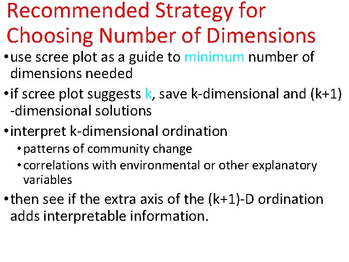
Recommended Strategy for Choosing Number of Dimensions • use scree plot as a guide to minimum number of dimensions needed • if scree plot suggests k, save k-dimensional and (k+1) -dimensional solutions • interpret k-dimensional ordination • patterns of community change • correlations with environmental or other explanatory variables • then see if the extra axis of the (k+1)-D ordination adds interpretable information.

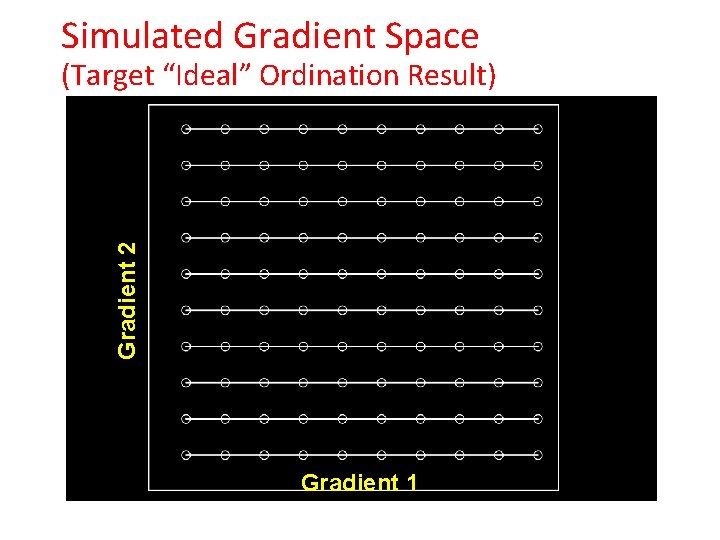
Simulated Gradient Space Gradient 2 (Target “Ideal” Ordination Result) Gradient 1

NMDS =0. 13 DCA =0. 09 CA =0. 10

NMDS =0. 08 DCA =0. 19 CA =0. 16

NMDS =0. 08 DCA =0. 19 CA =0. 29

NMDS =0. 09 DCA =0. 34 CA =0. 29

Treatment of Tied Dissimilarities • Kruskal noted that there are two ways to treat tied dissimilarities • Primary approach: pairs of SUs with equal dissimilarities need not be equally distant in the ordination • Secondary approach: pairs of SUs with equal dissimilarities should be equally distant in the ordination.

Treatment of Tied Dissimilarities • For community data, it is essential to use the primary approach, especially for SU pairs with no species in common (dissimilarity = 1. 0) • Such pairs of SUs generally have different environmental distances • Primary tie treatment allows NMDS to correctly estimate their distances • Use of secondary approach forces NMDS to represent gradients of high beta diversity as horseshoes.

mono. MDS {vegan} Global and Local Non-metric Multidimensional Scaling and Linear and Hybrid Scaling Description Function implements Kruskal's (1964 a, b) non-metric multidimensional scaling (NMDS) using monotone regression and primary (“weak”) treatment of ties. In addition to traditional global NMDS, the function implements local NMDS, linear and hybrid multidimensional scaling.

meta. MDS {vegan} Nonmetric Multidimensional Scaling with Stable Solution from Random Starts, Axis Scaling and Species Scores Description Function meta. MDS performs Nonmetric Multidimensional Scaling (NMDS), and tries to find a stable solution using several random starts. In addition, it standardizes the scaling in the result, so that the configurations are easier to interpret, and adds species scores to the site ordination. The meta. MDS function does not provide actual NMDS, but it calls another function for the purpose.