Algorithm Efficiency and Sorting Walls Mirrors Remainder of

Algorithm Efficiency and Sorting (Walls & Mirrors - Remainder of Chapter 9) 1

Overview • Mergesort • Quicksort th • Finding the K Smallest Item • Radix Sort 2

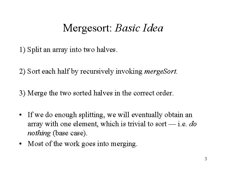
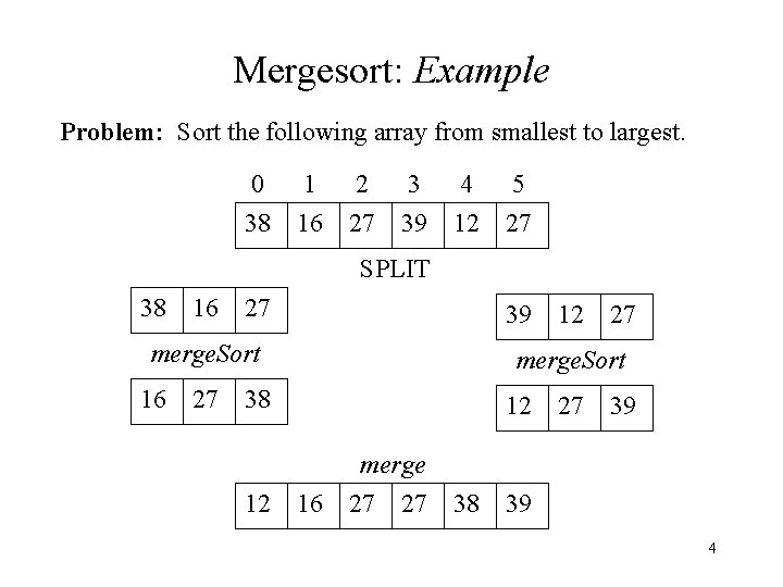
Mergesort: Basic Idea 1) Split an array into two halves. 2) Sort each half by recursively invoking merge. Sort. 3) Merge the two sorted halves in the correct order. • If we do enough splitting, we will eventually obtain an array with one element, which is trivial to sort — i. e. do nothing (base case). • Most of the work goes into merging. 3

Mergesort: Example Problem: Sort the following array from smallest to largest. 0 1 2 3 4 5 38 16 27 39 12 27 SPLIT 38 16 27 39 merge. Sort 16 27 27 merge. Sort 38 12 12 12 16 merge 27 27 38 27 39 39 4

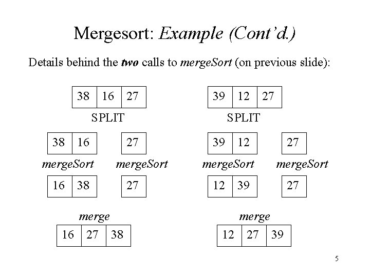
Mergesort: Example (Cont’d. ) Details behind the two calls to merge. Sort (on previous slide): 38 16 27 39 SPLIT 38 16 merge. Sort 27 merge 16 27 27 SPLIT 27 38 12 39 12 merge. Sort 12 27 merge. Sort 39 27 merge 38 12 27 39 5

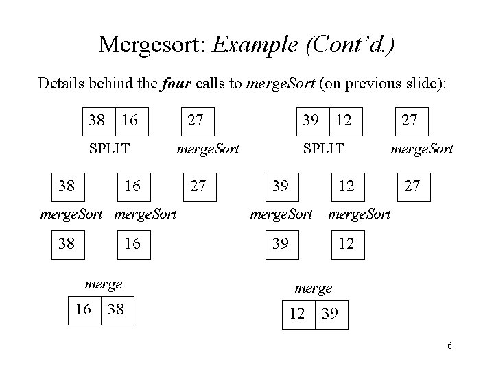
Mergesort: Example (Cont’d. ) Details behind the four calls to merge. Sort (on previous slide): 38 16 SPLIT 38 27 merge. Sort 16 merge. Sort 38 16 merge 16 38 39 12 27 SPLIT 39 27 merge. Sort 12 merge. Sort 27 merge. Sort 39 12 merge 12 39 6

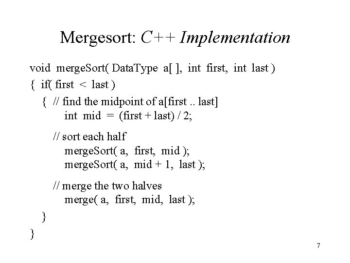
Mergesort: C++ Implementation void merge. Sort( Data. Type a[ ], int first, int last ) { if( first < last ) { // find the midpoint of a[first. . last] int mid = (first + last) / 2; // sort each half merge. Sort( a, first, mid ); merge. Sort( a, mid + 1, last ); // merge the two halves merge( a, first, mid, last ); } } 7

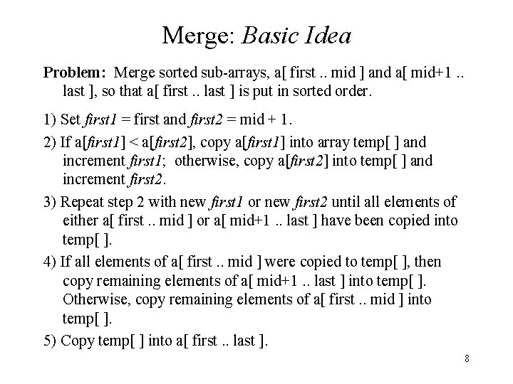
Merge: Basic Idea Problem: Merge sorted sub-arrays, a[ first. . mid ] and a[ mid+1. . last ], so that a[ first. . last ] is put in sorted order. 1) Set first 1 = first and first 2 = mid + 1. 2) If a[first 1] < a[first 2], copy a[first 1] into array temp[ ] and increment first 1; otherwise, copy a[first 2] into temp[ ] and increment first 2. 3) Repeat step 2 with new first 1 or new first 2 until all elements of either a[ first. . mid ] or a[ mid+1. . last ] have been copied into temp[ ]. 4) If all elements of a[ first. . mid ] were copied to temp[ ], then copy remaining elements of a[ mid+1. . last ] into temp[ ]. Otherwise, copy remaining elements of a[ first. . mid ] into temp[ ]. 5) Copy temp[ ] into a[ first. . last ]. 8

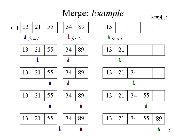
Merge: Example a[ ]: 13 21 55 first 1 34 89 first 2 temp[ ]: 13 index 13 21 55 34 89 13 21 34 55 89 9

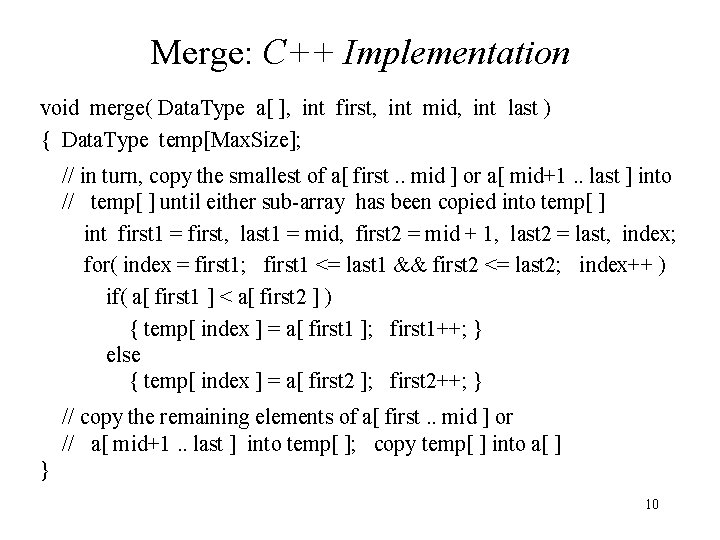
Merge: C++ Implementation void merge( Data. Type a[ ], int first, int mid, int last ) { Data. Type temp[Max. Size]; // in turn, copy the smallest of a[ first. . mid ] or a[ mid+1. . last ] into // temp[ ] until either sub-array has been copied into temp[ ] int first 1 = first, last 1 = mid, first 2 = mid + 1, last 2 = last, index; for( index = first 1; first 1 <= last 1 && first 2 <= last 2; index++ ) if( a[ first 1 ] < a[ first 2 ] ) { temp[ index ] = a[ first 1 ]; first 1++; } else { temp[ index ] = a[ first 2 ]; first 2++; } // copy the remaining elements of a[ first. . mid ] or // a[ mid+1. . last ] into temp[ ]; copy temp[ ] into a[ ] } 10

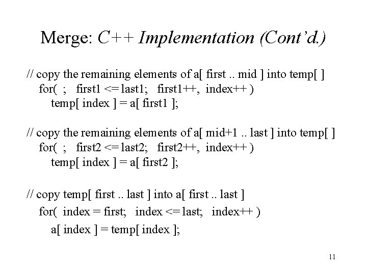
Merge: C++ Implementation (Cont’d. ) // copy the remaining elements of a[ first. . mid ] into temp[ ] for( ; first 1 <= last 1; first 1++, index++ ) temp[ index ] = a[ first 1 ]; // copy the remaining elements of a[ mid+1. . last ] into temp[ ] for( ; first 2 <= last 2; first 2++, index++ ) temp[ index ] = a[ first 2 ]; // copy temp[ first. . last ] into a[ first. . last ] for( index = first; index <= last; index++ ) a[ index ] = temp[ index ]; 11

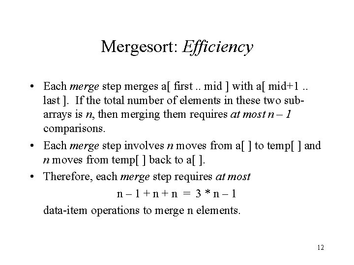
Mergesort: Efficiency • Each merge step merges a[ first. . mid ] with a[ mid+1. . last ]. If the total number of elements in these two subarrays is n, then merging them requires at most n – 1 comparisons. • Each merge step involves n moves from a[ ] to temp[ ] and n moves from temp[ ] back to a[ ]. • Therefore, each merge step requires at most n– 1+n+n = 3*n– 1 data-item operations to merge n elements. 12

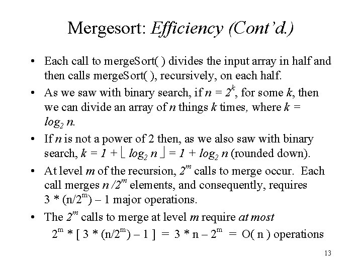
Mergesort: Efficiency (Cont’d. ) • Each call to merge. Sort( ) divides the input array in half and then calls merge. Sort( ), recursively, on each half. • As we saw with binary search, if n = 2 k, for some k, then we can divide an array of n things k times, where k = log 2 n. • If n is not a power of 2 then, as we also saw with binary search, k = 1 + log 2 n = 1 + log 2 n (rounded down). • At level m of the recursion, 2 m calls to merge occur. Each call merges n /2 m elements, and consequently, requires 3 * (n/2 m) – 1 major operations. • The 2 m calls to merge at level m require at most 2 m * [ 3 * (n/2 m) – 1 ] = 3 * n – 2 m = O( n ) operations 13

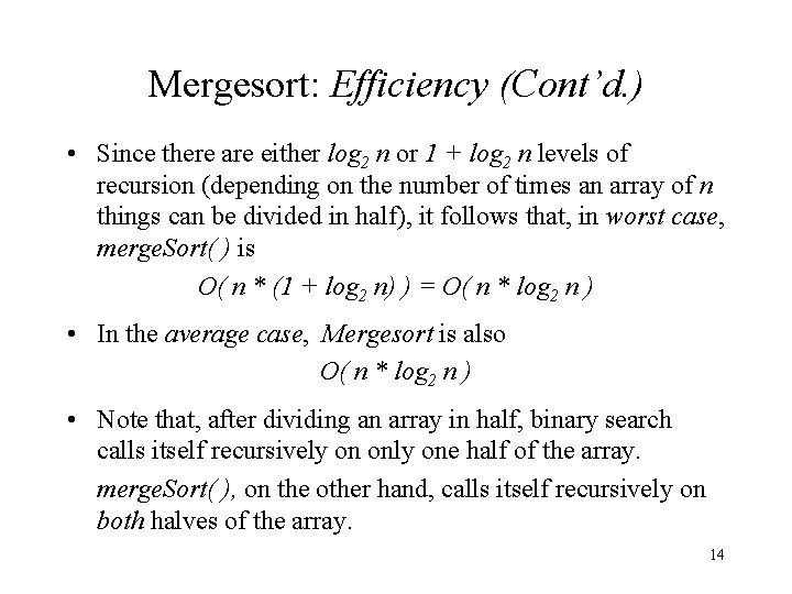
Mergesort: Efficiency (Cont’d. ) • Since there are either log 2 n or 1 + log 2 n levels of recursion (depending on the number of times an array of n things can be divided in half), it follows that, in worst case, merge. Sort( ) is O( n * (1 + log 2 n) ) = O( n * log 2 n ) • In the average case, Mergesort is also O( n * log 2 n ) • Note that, after dividing an array in half, binary search calls itself recursively on only one half of the array. merge. Sort( ), on the other hand, calls itself recursively on both halves of the array. 14

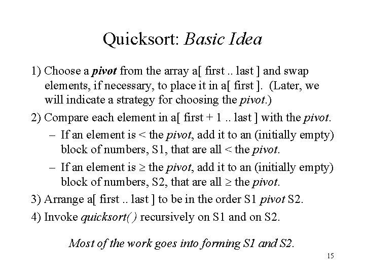
Quicksort: Basic Idea 1) Choose a pivot from the array a[ first. . last ] and swap elements, if necessary, to place it in a[ first ]. (Later, we will indicate a strategy for choosing the pivot. ) 2) Compare each element in a[ first + 1. . last ] with the pivot. – If an element is < the pivot, add it to an (initially empty) block of numbers, S 1, that are all < the pivot. – If an element is the pivot, add it to an (initially empty) block of numbers, S 2, that are all the pivot. 3) Arrange a[ first. . last ] to be in the order S 1 pivot S 2. 4) Invoke quicksort( ) recursively on S 1 and on S 2. Most of the work goes into forming S 1 and S 2. 15

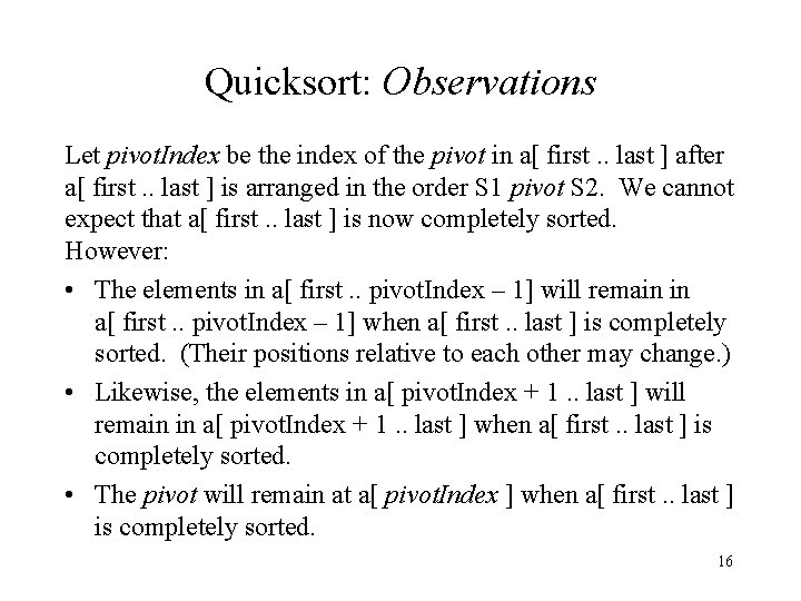
Quicksort: Observations Let pivot. Index be the index of the pivot in a[ first. . last ] after a[ first. . last ] is arranged in the order S 1 pivot S 2. We cannot expect that a[ first. . last ] is now completely sorted. However: • The elements in a[ first. . pivot. Index – 1] will remain in a[ first. . pivot. Index – 1] when a[ first. . last ] is completely sorted. (Their positions relative to each other may change. ) • Likewise, the elements in a[ pivot. Index + 1. . last ] will remain in a[ pivot. Index + 1. . last ] when a[ first. . last ] is completely sorted. • The pivot will remain at a[ pivot. Index ] when a[ first. . last ] is completely sorted. 16

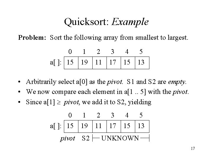
Quicksort: Example Problem: Sort the following array from smallest to largest. 0 1 2 3 4 5 a[ ]: 15 19 11 17 15 13 • Arbitrarily select a[0] as the pivot. S 1 and S 2 are empty. • We now compare each element in a[1. . 5] with the pivot. • Since a[1] pivot, we add it to S 2, yielding 0 a[ ]: 15 1 19 pivot S 2 2 3 11 17 4 15 5 13 UNKNOWN 17

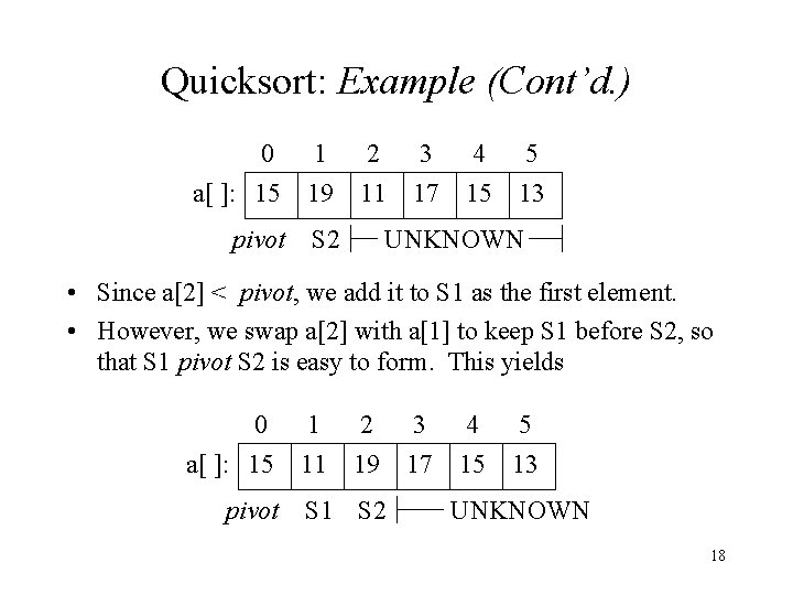
Quicksort: Example (Cont’d. ) 0 1 2 3 4 5 a[ ]: 15 19 11 17 15 13 pivot S 2 UNKNOWN • Since a[2] < pivot, we add it to S 1 as the first element. • However, we swap a[2] with a[1] to keep S 1 before S 2, so that S 1 pivot S 2 is easy to form. This yields 0 1 2 3 4 5 a[ ]: 15 11 19 17 15 13 pivot S 1 S 2 UNKNOWN 18

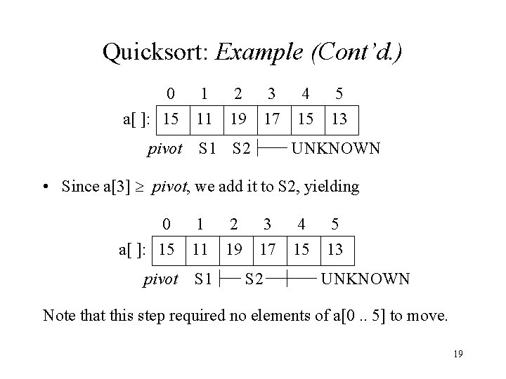
Quicksort: Example (Cont’d. ) 0 1 2 3 4 5 a[ ]: 15 11 19 17 15 13 pivot S 1 S 2 UNKNOWN • Since a[3] pivot, we add it to S 2, yielding 0 1 2 3 4 5 a[ ]: 15 11 19 17 15 13 pivot S 1 S 2 UNKNOWN Note that this step required no elements of a[0. . 5] to move. 19

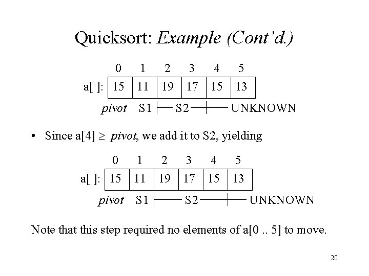
Quicksort: Example (Cont’d. ) 0 1 3 4 5 a[ ]: 15 11 19 17 15 13 pivot S 2 S 1 2 UNKNOWN • Since a[4] pivot, we add it to S 2, yielding 0 a[ ]: 15 1 11 2 3 19 17 pivot S 1 S 2 4 15 5 13 UNKNOWN Note that this step required no elements of a[0. . 5] to move. 20

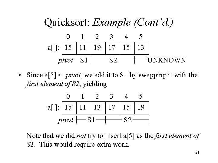
Quicksort: Example (Cont’d. ) 0 1 2 3 4 5 a[ ]: 15 11 19 17 15 13 pivot S 1 S 2 UNKNOWN • Since a[5] < pivot, we add it to S 1 by swapping it with the first element of S 2, yielding 0 a[ ]: 15 pivot 1 11 2 3 13 17 S 1 4 15 5 19 S 2 Note that we did not try to insert a[5] as the first element of S 1. This would require extra work. 21

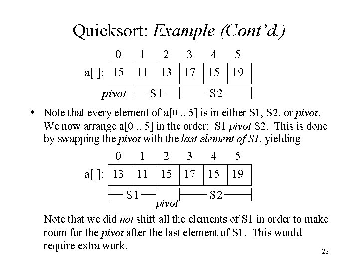
Quicksort: Example (Cont’d. ) 0 1 2 3 4 5 a[ ]: 15 11 13 17 15 19 pivot S 1 S 2 • Note that every element of a[0. . 5] is in either S 1, S 2, or pivot. We now arrange a[0. . 5] in the order: S 1 pivot S 2. This is done by swapping the pivot with the last element of S 1, yielding 0 a[ ]: 13 1 11 S 1 2 3 15 17 4 15 S 2 5 19 pivot Note that we did not shift all the elements of S 1 in order to make room for the pivot after the last element of S 1. This would require extra work. 22

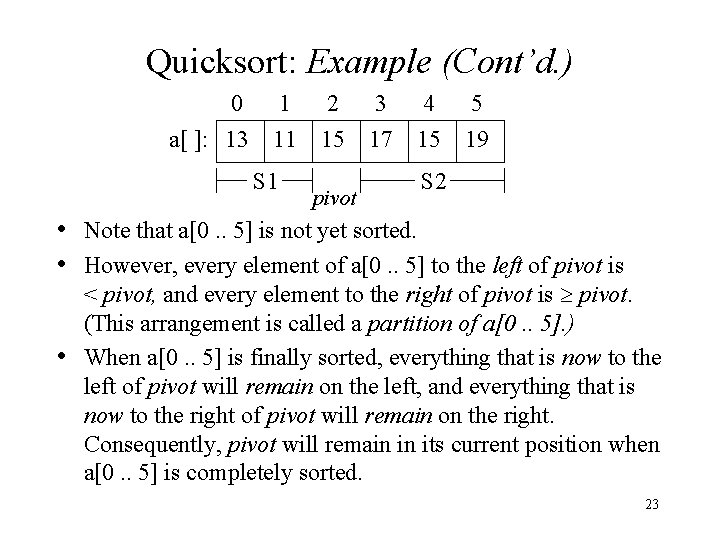
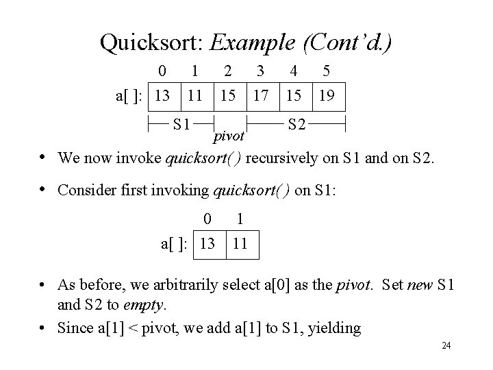
Quicksort: Example (Cont’d. ) 0 1 2 3 4 5 a[ ]: 13 11 15 17 15 19 S 1 pivot S 2 • Note that a[0. . 5] is not yet sorted. • However, every element of a[0. . 5] to the left of pivot is • < pivot, and every element to the right of pivot is pivot. (This arrangement is called a partition of a[0. . 5]. ) When a[0. . 5] is finally sorted, everything that is now to the left of pivot will remain on the left, and everything that is now to the right of pivot will remain on the right. Consequently, pivot will remain in its current position when a[0. . 5] is completely sorted. 23

Quicksort: Example (Cont’d. ) 0 1 2 3 4 5 a[ ]: 13 11 15 17 15 19 S 1 pivot S 2 • We now invoke quicksort( ) recursively on S 1 and on S 2. • Consider first invoking quicksort( ) on S 1: 0 a[ ]: 13 1 11 • As before, we arbitrarily select a[0] as the pivot. Set new S 1 and S 2 to empty. • Since a[1] < pivot, we add a[1] to S 1, yielding 24

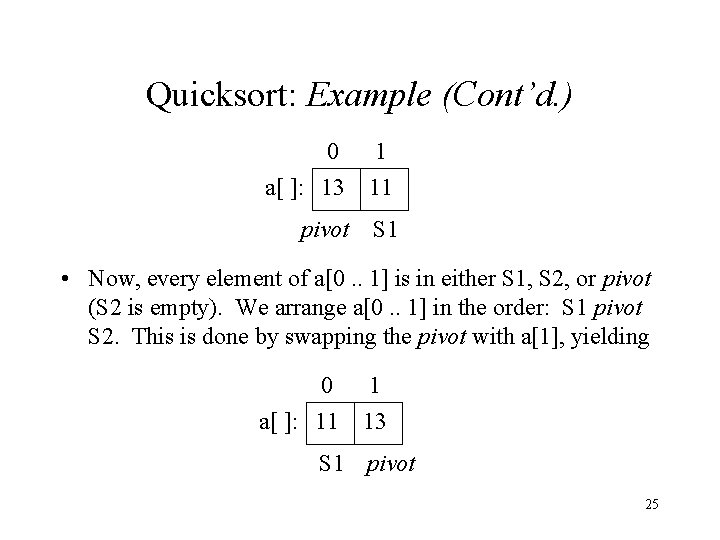
Quicksort: Example (Cont’d. ) 0 1 a[ ]: 13 11 pivot S 1 • Now, every element of a[0. . 1] is in either S 1, S 2, or pivot (S 2 is empty). We arrange a[0. . 1] in the order: S 1 pivot S 2. This is done by swapping the pivot with a[1], yielding 0 a[ ]: 11 1 13 S 1 pivot 25

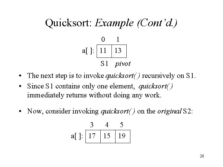
Quicksort: Example (Cont’d. ) 0 1 a[ ]: 11 13 S 1 pivot • The next step is to invoke quicksort( ) recursively on S 1. • Since S 1 contains only one element, quicksort( ) immediately returns without doing any work. • Now, consider invoking quicksort( ) on the original S 2: 3 4 5 a[ ]: 17 15 19 26

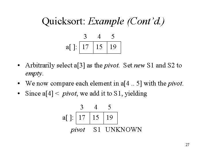
Quicksort: Example (Cont’d. ) 3 4 5 a[ ]: 17 15 19 • Arbitrarily select a[3] as the pivot. Set new S 1 and S 2 to empty. • We now compare each element in a[4. . 5] with the pivot. • Since a[4] < pivot, we add it to S 1, yielding 3 4 5 a[ ]: 17 15 19 pivot S 1 UNKNOWN 27

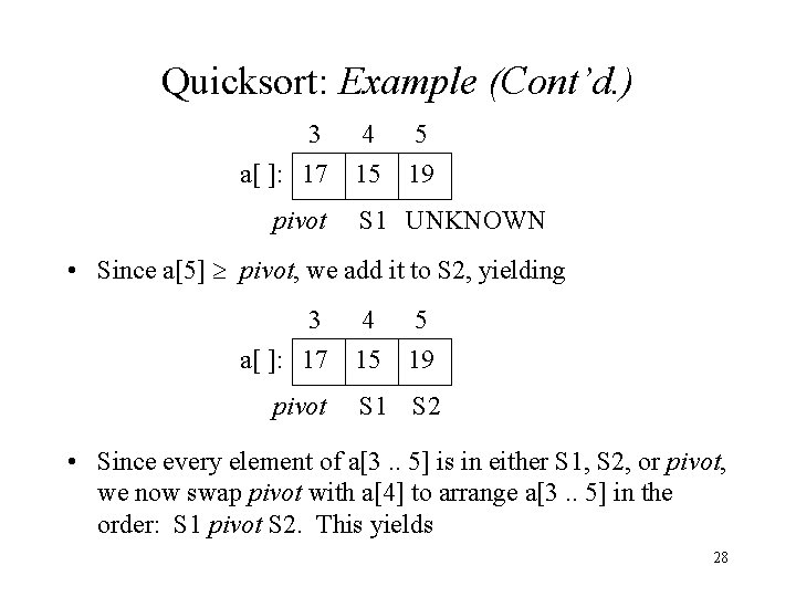
Quicksort: Example (Cont’d. ) 3 4 5 a[ ]: 17 15 19 pivot S 1 UNKNOWN • Since a[5] pivot, we add it to S 2, yielding 3 4 5 a[ ]: 17 15 19 pivot S 1 S 2 • Since every element of a[3. . 5] is in either S 1, S 2, or pivot, we now swap pivot with a[4] to arrange a[3. . 5] in the order: S 1 pivot S 2. This yields 28

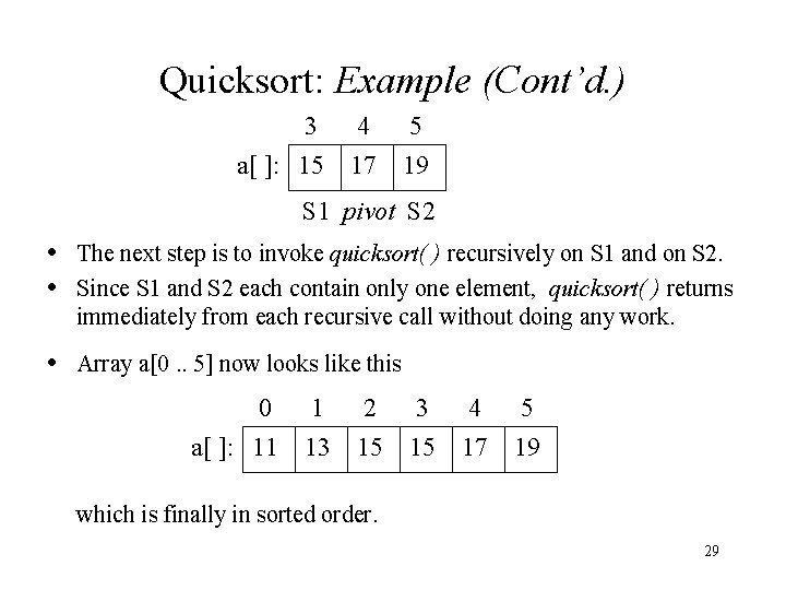
Quicksort: Example (Cont’d. ) 3 4 5 a[ ]: 15 17 19 S 1 pivot S 2 • The next step is to invoke quicksort( ) recursively on S 1 and on S 2. • Since S 1 and S 2 each contain only one element, quicksort( ) returns immediately from each recursive call without doing any work. • Array a[0. . 5] now looks like this 0 a[ ]: 11 1 13 2 3 15 15 4 17 5 19 which is finally in sorted order. 29

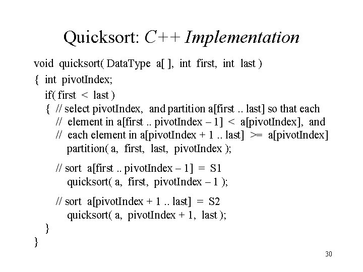
Quicksort: C++ Implementation void quicksort( Data. Type a[ ], int first, int last ) { int pivot. Index; if( first < last ) { // select pivot. Index, and partition a[first. . last] so that each // element in a[first. . pivot. Index – 1] < a[pivot. Index], and // each element in a[pivot. Index + 1. . last] >= a[pivot. Index] partition( a, first, last, pivot. Index ); // sort a[first. . pivot. Index – 1] = S 1 quicksort( a, first, pivot. Index – 1 ); // sort a[pivot. Index + 1. . last] = S 2 quicksort( a, pivot. Index + 1, last ); } } 30

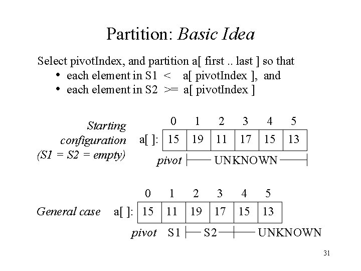
Partition: Basic Idea Select pivot. Index, and partition a[ first. . last ] so that • each element in S 1 < a[ pivot. Index ], and • each element in S 2 >= a[ pivot. Index ] Starting configuration (S 1 = S 2 = empty) General case 0 1 2 3 4 5 a[ ]: 15 19 11 17 15 13 pivot 0 1 a[ ]: 15 11 pivot S 1 UNKNOWN 2 19 3 17 S 2 4 15 5 13 UNKNOWN 31

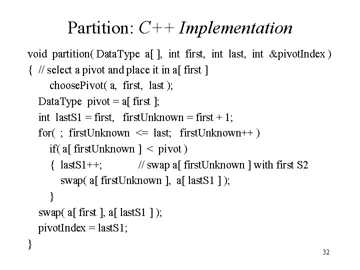
Partition: C++ Implementation void partition( Data. Type a[ ], int first, int last, int &pivot. Index ) { // select a pivot and place it in a[ first ] choose. Pivot( a, first, last ); Data. Type pivot = a[ first ]; int last. S 1 = first, first. Unknown = first + 1; for( ; first. Unknown <= last; first. Unknown++ ) if( a[ first. Unknown ] < pivot ) { last. S 1++; // swap a[ first. Unknown ] with first S 2 swap( a[ first. Unknown ], a[ last. S 1 ] ); } swap( a[ first ], a[ last. S 1 ] ); pivot. Index = last. S 1; } 32

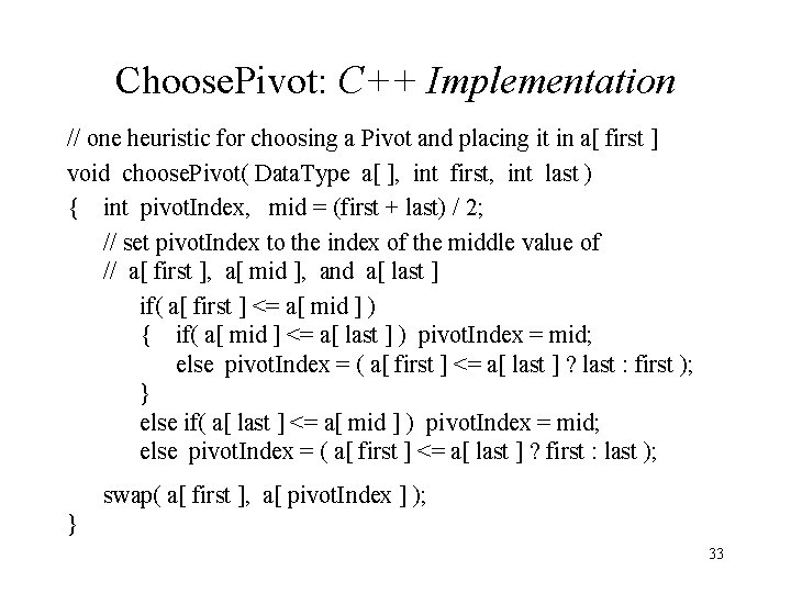
Choose. Pivot: C++ Implementation // one heuristic for choosing a Pivot and placing it in a[ first ] void choose. Pivot( Data. Type a[ ], int first, int last ) { int pivot. Index, mid = (first + last) / 2; // set pivot. Index to the index of the middle value of // a[ first ], a[ mid ], and a[ last ] if( a[ first ] <= a[ mid ] ) { if( a[ mid ] <= a[ last ] ) pivot. Index = mid; else pivot. Index = ( a[ first ] <= a[ last ] ? last : first ); } else if( a[ last ] <= a[ mid ] ) pivot. Index = mid; else pivot. Index = ( a[ first ] <= a[ last ] ? first : last ); swap( a[ first ], a[ pivot. Index ] ); } 33

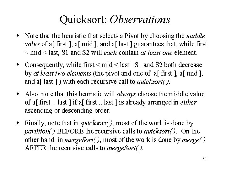
Quicksort: Observations • Note that the heuristic that selects a Pivot by choosing the middle value of a[ first ], a[ mid ], and a[ last ] guarantees that, while first < mid < last, S 1 and S 2 will each contain at least one element. • Consequently, while first < mid < last, S 1 and S 2 both decrease by at least two elements (the pivot and one of a[ first ], a[ mid ], and a[ last ] ) with each recursive call to quicksort( ). • Also, note that this heuristic will always choose the middle value of a[ first. . last ] is already arranged in either ascending or descending order. • Finally, note that in quicksort( ), most of the work is done by partition( ) BEFORE the recursive calls to quicksort( ). On the other hand, in merge. Sort( ), most of the work is done by merge( ) AFTER the recursive calls to merge. Sort( ). 34

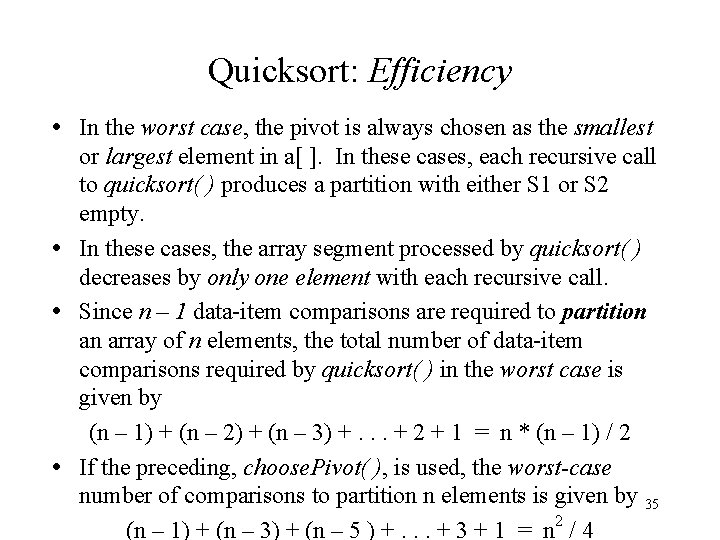
Quicksort: Efficiency • In the worst case, the pivot is always chosen as the smallest or largest element in a[ ]. In these cases, each recursive call to quicksort( ) produces a partition with either S 1 or S 2 empty. • In these cases, the array segment processed by quicksort( ) decreases by only one element with each recursive call. • Since n – 1 data-item comparisons are required to partition an array of n elements, the total number of data-item comparisons required by quicksort( ) in the worst case is given by (n – 1) + (n – 2) + (n – 3) +. . . + 2 + 1 = n * (n – 1) / 2 • If the preceding, choose. Pivot( ), is used, the worst-case number of comparisons to partition n elements is given by 35 (n – 1) + (n – 3) + (n – 5 ) +. . . + 3 + 1 = n 2 / 4

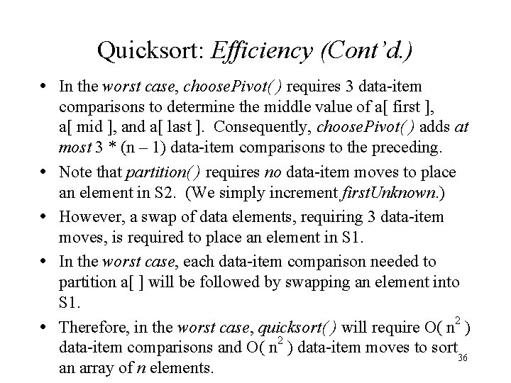
Quicksort: Efficiency (Cont’d. ) • In the worst case, choose. Pivot( ) requires 3 data-item • • comparisons to determine the middle value of a[ first ], a[ mid ], and a[ last ]. Consequently, choose. Pivot( ) adds at most 3 * (n – 1) data-item comparisons to the preceding. Note that partition( ) requires no data-item moves to place an element in S 2. (We simply increment first. Unknown. ) However, a swap of data elements, requiring 3 data-item moves, is required to place an element in S 1. In the worst case, each data-item comparison needed to partition a[ ] will be followed by swapping an element into S 1. Therefore, in the worst case, quicksort( ) will require O( n 2 ) data-item comparisons and O( n 2 ) data-item moves to sort 36 an array of n elements.

Quicksort: Summary • In the worst case, Quicksort requires O( n 2 ) time to sort an array of n elements, similar to Insertion sort, Selection sort, and Bubble sort. • Further analysis shows that Quicksort’s average running time is O( n * log 2 n ), like Mergesort. • However, in practice, Quicksort usually runs faster than Mergesort, and Quicksort does not need the extra space for a temporary array as Mergesort does. 37

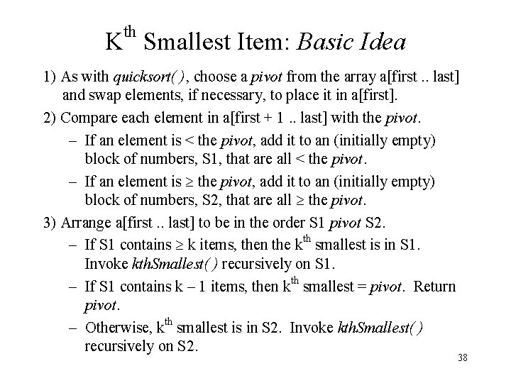
th K Smallest Item: Basic Idea 1) As with quicksort( ), choose a pivot from the array a[first. . last] and swap elements, if necessary, to place it in a[first]. 2) Compare each element in a[first + 1. . last] with the pivot. – If an element is < the pivot, add it to an (initially empty) block of numbers, S 1, that are all < the pivot. – If an element is the pivot, add it to an (initially empty) block of numbers, S 2, that are all the pivot. 3) Arrange a[first. . last] to be in the order S 1 pivot S 2. – If S 1 contains k items, then the kth smallest is in S 1. Invoke kth. Smallest( ) recursively on S 1. – If S 1 contains k – 1 items, then kth smallest = pivot. Return pivot. – Otherwise, kth smallest is in S 2. Invoke kth. Smallest( ) recursively on S 2. 38

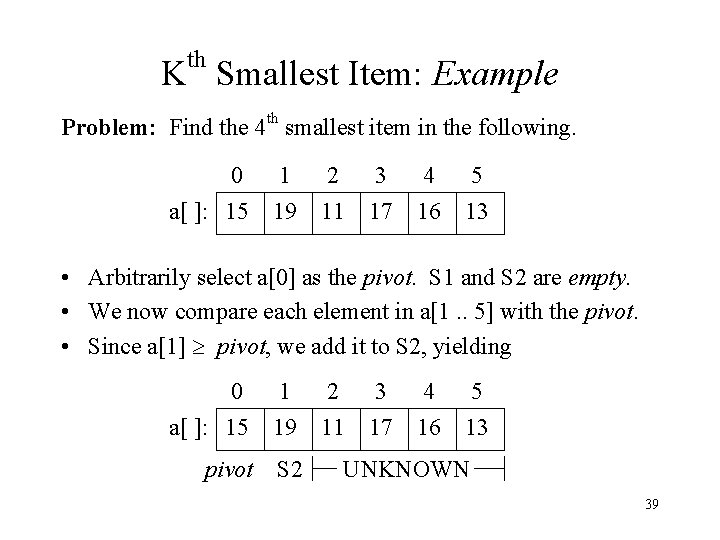
th K Smallest Item: Example th Problem: Find the 4 smallest item in the following. 0 1 2 3 4 5 a[ ]: 15 19 11 17 16 13 • Arbitrarily select a[0] as the pivot. S 1 and S 2 are empty. • We now compare each element in a[1. . 5] with the pivot. • Since a[1] pivot, we add it to S 2, yielding 0 a[ ]: 15 1 19 pivot S 2 2 3 11 17 4 16 5 13 UNKNOWN 39

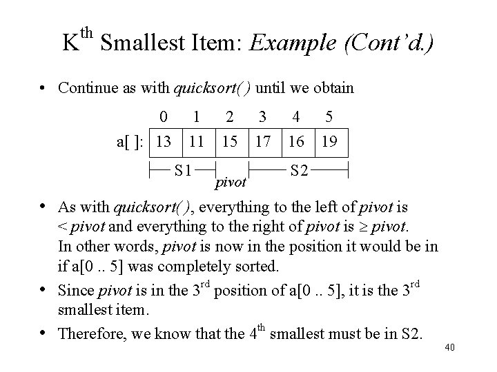
th K Smallest Item: Example (Cont’d. ) • Continue as with quicksort( ) until we obtain 0 1 2 3 4 5 a[ ]: 13 11 15 17 16 19 S 1 pivot S 2 • As with quicksort( ), everything to the left of pivot is • • < pivot and everything to the right of pivot is pivot. In other words, pivot is now in the position it would be in if a[0. . 5] was completely sorted. Since pivot is in the 3 rd position of a[0. . 5], it is the 3 rd smallest item. Therefore, we know that the 4 th smallest must be in S 2. 40

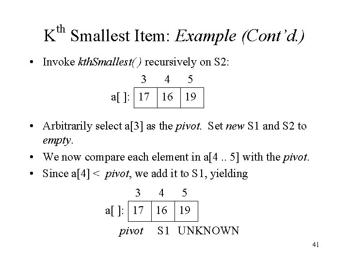
th K Smallest Item: Example (Cont’d. ) • Invoke kth. Smallest( ) recursively on S 2: 3 4 5 a[ ]: 17 16 19 • Arbitrarily select a[3] as the pivot. Set new S 1 and S 2 to empty. • We now compare each element in a[4. . 5] with the pivot. • Since a[4] < pivot, we add it to S 1, yielding 3 4 5 a[ ]: 17 16 19 pivot S 1 UNKNOWN 41

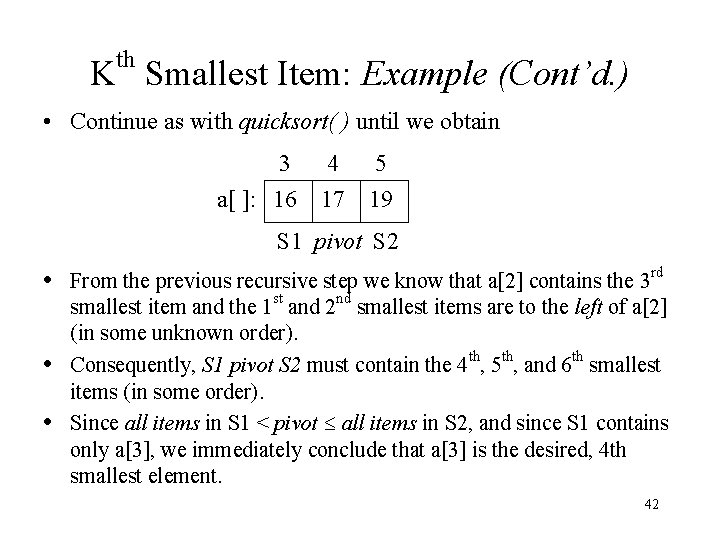
th K Smallest Item: Example (Cont’d. ) • Continue as with quicksort( ) until we obtain 3 4 5 a[ ]: 16 17 19 S 1 pivot S 2 • From the previous recursive step we know that a[2] contains the 3 rd • • smallest item and the 1 st and 2 nd smallest items are to the left of a[2] (in some unknown order). Consequently, S 1 pivot S 2 must contain the 4 th, 5 th, and 6 th smallest items (in some order). Since all items in S 1 < pivot all items in S 2, and since S 1 contains only a[3], we immediately conclude that a[3] is the desired, 4 th smallest element. 42

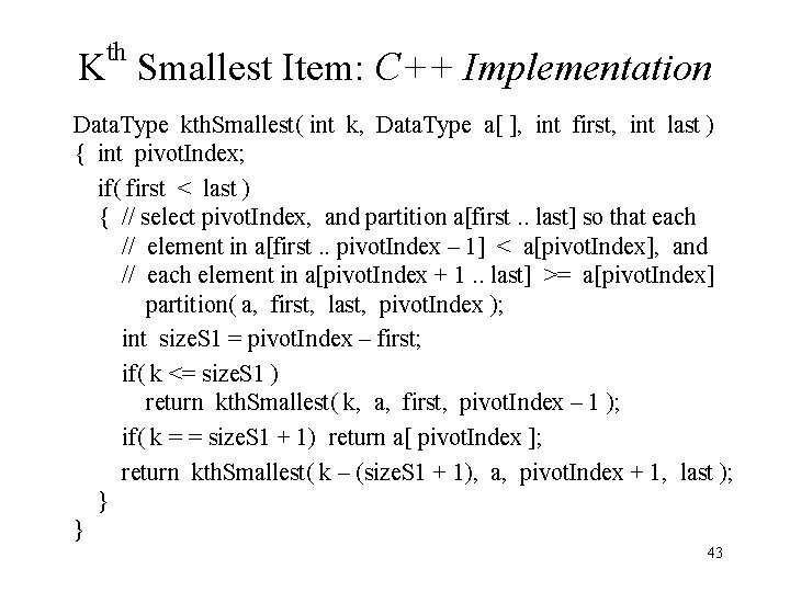
th K Smallest Item: C++ Implementation Data. Type kth. Smallest( int k, Data. Type a[ ], int first, int last ) { int pivot. Index; if( first < last ) { // select pivot. Index, and partition a[first. . last] so that each // element in a[first. . pivot. Index – 1] < a[pivot. Index], and // each element in a[pivot. Index + 1. . last] >= a[pivot. Index] partition( a, first, last, pivot. Index ); int size. S 1 = pivot. Index – first; if( k <= size. S 1 ) return kth. Smallest( k, a, first, pivot. Index – 1 ); if( k = = size. S 1 + 1) return a[ pivot. Index ]; return kth. Smallest( k – (size. S 1 + 1), a, pivot. Index + 1, last ); } } 43

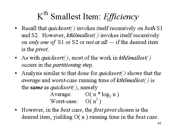
th K Smallest Item: Efficiency • Recall that quicksort( ) invokes itself recursively on both S 1 and S 2. However, kth. Smallest( ) invokes itself recursively on only one of S 1 or S 2 or not at all — if the desired item is the pivot. • As with quicksort( ), most of the work in kth. Smallest( ) occurs in the partitioning step. • Analysis similar to that done for quicksort( ) shows that the average and worst-case running time of kth. Smallest( ) is the same as quicksort( ), namely Average: O( n * log 2 n ) Worst-case: O( n 2 ) • However, in the best case, the first pivot chosen is the desired item, yielding O( n ) running time in the best case. 44

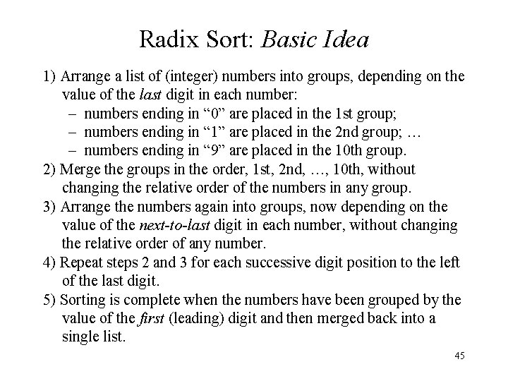
Radix Sort: Basic Idea 1) Arrange a list of (integer) numbers into groups, depending on the value of the last digit in each number: – numbers ending in “ 0” are placed in the 1 st group; – numbers ending in “ 1” are placed in the 2 nd group; … – numbers ending in “ 9” are placed in the 10 th group. 2) Merge the groups in the order, 1 st, 2 nd, …, 10 th, without changing the relative order of the numbers in any group. 3) Arrange the numbers again into groups, now depending on the value of the next-to-last digit in each number, without changing the relative order of any number. 4) Repeat steps 2 and 3 for each successive digit position to the left of the last digit. 5) Sorting is complete when the numbers have been grouped by the value of the first (leading) digit and then merged back into a single list. 45

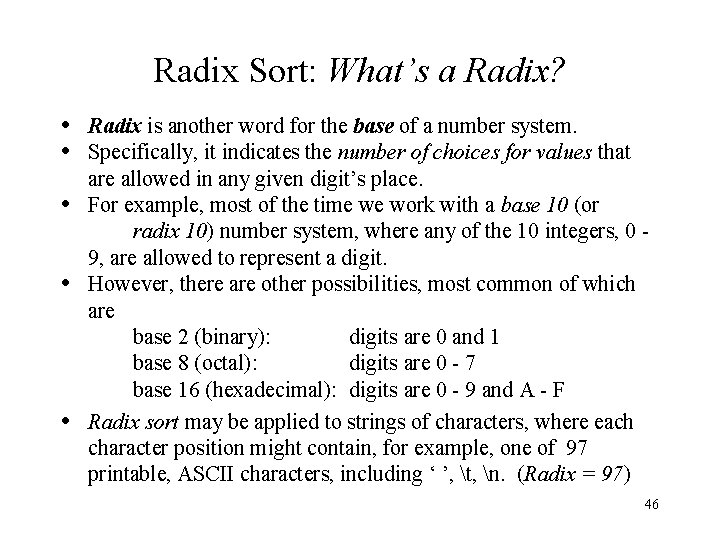
Radix Sort: What’s a Radix? • Radix is another word for the base of a number system. • Specifically, it indicates the number of choices for values that • • • are allowed in any given digit’s place. For example, most of the time we work with a base 10 (or radix 10) number system, where any of the 10 integers, 0 9, are allowed to represent a digit. However, there are other possibilities, most common of which are base 2 (binary): digits are 0 and 1 base 8 (octal): digits are 0 - 7 base 16 (hexadecimal): digits are 0 - 9 and A - F Radix sort may be applied to strings of characters, where each character position might contain, for example, one of 97 printable, ASCII characters, including ‘ ’, t, n. (Radix = 97) 46

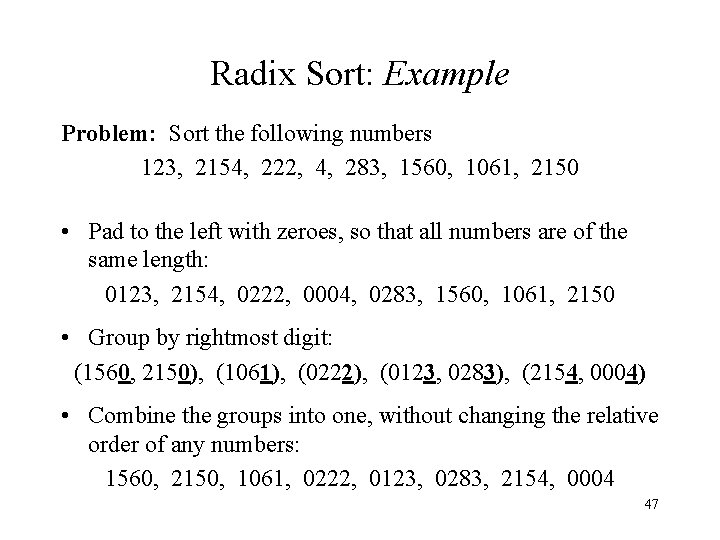
Radix Sort: Example Problem: Sort the following numbers 123, 2154, 222, 4, 283, 1560, 1061, 2150 • Pad to the left with zeroes, so that all numbers are of the same length: 0123, 2154, 0222, 0004, 0283, 1560, 1061, 2150 • Group by rightmost digit: (1560, 2150), (1061), (0222), (0123, 0283), (2154, 0004) • Combine the groups into one, without changing the relative order of any numbers: 1560, 2150, 1061, 0222, 0123, 0283, 2154, 0004 47

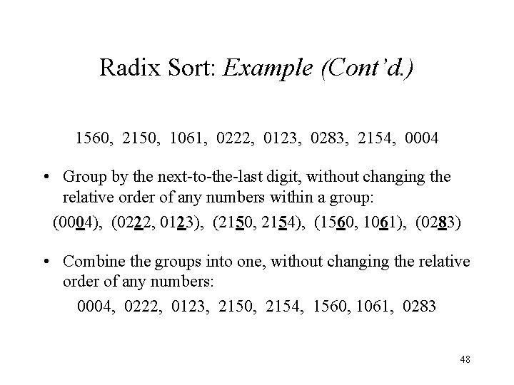
Radix Sort: Example (Cont’d. ) 1560, 2150, 1061, 0222, 0123, 0283, 2154, 0004 • Group by the next-to-the-last digit, without changing the relative order of any numbers within a group: (0004), (0222, 0123), (2150, 2154), (1560, 1061), (0283) • Combine the groups into one, without changing the relative order of any numbers: 0004, 0222, 0123, 2150, 2154, 1560, 1061, 0283 48

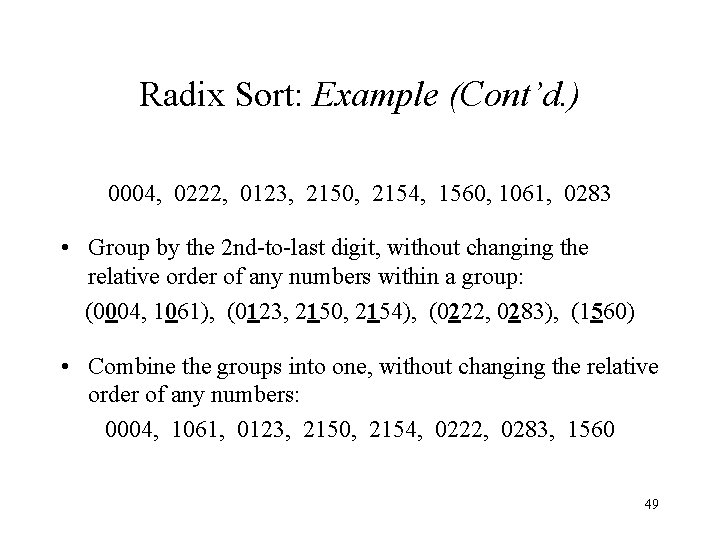
Radix Sort: Example (Cont’d. ) 0004, 0222, 0123, 2150, 2154, 1560, 1061, 0283 • Group by the 2 nd-to-last digit, without changing the relative order of any numbers within a group: (0004, 1061), (0123, 2150, 2154), (0222, 0283), (1560) • Combine the groups into one, without changing the relative order of any numbers: 0004, 1061, 0123, 2150, 2154, 0222, 0283, 1560 49

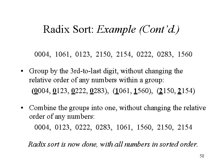
Radix Sort: Example (Cont’d. ) 0004, 1061, 0123, 2150, 2154, 0222, 0283, 1560 • Group by the 3 rd-to-last digit, without changing the relative order of any numbers within a group: (0004, 0123, 0222, 0283), (1061, 1560), (2150, 2154) • Combine the groups into one, without changing the relative order of any numbers: 0004, 0123, 0222, 0283, 1061, 1560, 2154 Radix sort is now done, with all numbers in sorted order. 50

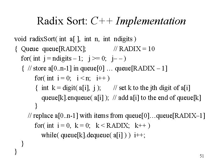
Radix Sort: C++ Implementation void radix. Sort( int a[ ], int ndigits ) { Queue queue[RADIX]; // RADIX = 10 for( int j = ndigits – 1; j >= 0; j– – ) { // store a[0. . n-1] in queue[0] … queue[RADIX – 1] for( int i = 0; i < n; i++ ) { int k = digit( a[i], j ); // set k to the jth digit of a[i] queue[k]. enqueue( a[i] ); // add a[i] to the end of queue[k] } // replace a[0. . n-1] with items from queue[0]…queue[RADIX– 1] for( int i = 0, k = 0; k < RADIX; k++ ) while( queue[k]. dequeue( a[i] ) ) i++; } } 51

Radix Sort: Efficiency • Note that Radix sort requires no data-item comparisons! • For each digit in a data item, Radix sort enqueues and dequeues n elements of a[ ]. • The number of data-item moves, therefore, is ndigits * n * 2 • For a given application, there is a constant, C, such that ndigits < C. (For example, for 32 -bit integers, C = 10. ) • Therefore, by this analysis, Radix sort requires O( n ) time to sort n items in the best, average, and worst cases. 52

Radix Sort: Efficiency Caveat • Although the preceding analysis is technically correct, a more • • careful analysis shows that the loop for( int i = 0, k = 0; k < RADIX; k++ ) while( queue[k]. dequeue( a[i] ) ) i++; executes dequeue( ) RADIX + n times. The running time of Radix sort is, therefore, proportional to ndigits * ( n + RADIX + n ) which is O( ndigits * ( RADIX + n ) ) Although for a given application, there are constants C 1 and C 2, such that ndigits < C 1 and RADIX < C 2, their impact cannot be ignored if either or both of them is large. (RADIX could be ~100 ( 256) for character strings, and ndigits could be 40 or more for RSA Security keys. ) 53

Radix Sort: Summary • Radix sort requires O( ndigits * ( RADIX + n )) = O( n ) time to • • • sort n items in the best, worst, and average cases. Radix sort requires no data-item comparisons. Radix sort requires that the data items all be of the same length. If the data items are integers, they are padded (to the left) with zeroes. If the data items are character strings, they are padded (to the right) with blanks. Radix sort requires extracting each digit from each data item, or n * ndigits extractions. (On a binary computer, this will be most efficient if the RADIX is a power of 2 — e. g. 2, 8 or 16. ) Radix sort requires extra storage and software to manage the queues that are required. (Number of queues = RADIX. ) For the three previous reasons, Radix sort can be somewhat awkward to use, in spite of its O( n ) running time. 54

Radix Sort: Summary (Cont’d. ) • In practice, it is sometimes sufficient to use Radix sort on the leading digits only (to form a set of queues), and then use some other method, such as Quicksort or Insertion sort, to sort the individual queues. 55

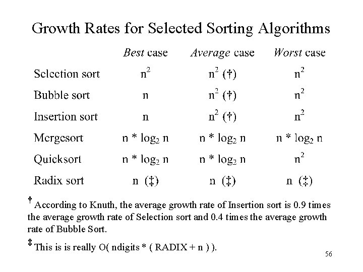
Growth Rates for Selected Sorting Algorithms † According to Knuth, the average growth rate of Insertion sort is 0. 9 times the average growth rate of Selection sort and 0. 4 times the average growth rate of Bubble Sort. ‡ This is is really O( ndigits * ( RADIX + n ) ). 56